


Logistic Regression
The data
我们将建立一个逻辑回归模型来预测一个学生是否被大学录取。假设你是一个大学系的管理员,你想根据两次考试的结果来决定每个申请人的录取机会。你有以前的申请人的历史数据,你可以用它作为逻辑回归的训练集。对于每一个培训例子,你有两个考试的申请人的分数和录取决定。为了做到这一点,我们将建立一个分类模型,根据考试成绩估计入学概率。
#导入三大件

import numpy as np

import pandas as pd

import matplotlib.pyplot as plt

%matplotlib inline

import os

path = 'data' + os.sep + 'LogiReg_data.txt'

pdData = pd.read_csv(path, header = None, names = ['Exam 1', 'Exam 2', 'Admitted'])

#查看通过申请和没有通过申请的数据的两项特征指标分布

positive = pdData[pdData['Admitted'] == 1]

negative = pdData[pdData['Admitted'] == 0]


fig,ax = plt.subplots(figsize = (10,5))

ax.scatter(postive['Exam 1'], positive['Exam 2'], s = 30, c = 'b', marker = 'o', label = 'Admitted')

ax.scatter(negative['Exam 1'], negative['Exam 2'], s = 30, c = 'r', marker = 'x', label = 'Not Admitted')

ax.legend()

ax.set_xlabel('Exam 1 Score')

ax.set_ylabel('Exam 2 Score')
The logistic regression
目标:建立分类器(求解出三个参数 𝜃0𝜃1𝜃2
)
设定阈值,根据阈值判断录取结果
要完成的模块
-
sigmoid: 映射到概率的函数 -
model: 返回预测结果值 -
cost: 根据参数计算损失 -
gradient: 计算每个参数的梯度方向 -
descent: 进行参数更新 -
accuracy: 计算精度
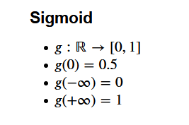
sigmoid 函数
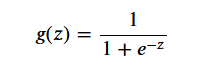
def sigmoid(z):
return 1 / (1+np.exp(-z))
#设置映射函数

def model(X, theta):
return sigmoid(np.dot(X, theta.T))
#构造预测函数其中theta为各特征变量的系数矩阵,X为样本数据或者是用来预测的数据的分数部分

pdData.insert(0, 'Ones', 1)
#拆入常数项对应的系数1,这里0是插入的列的序号
#设置X(训练数据)和y(目标变量)set X(training data) and y (target variable)
orig_data = pdData.as_matrix()
#将数据的panda表示转换为对进一步计算有用的数组
cols = orig_data.shape(1)
X = orig_data[:,0:cols-1]
y = orig_data[:,cols-1:cols]
theta = np.zeros([1,3])

def cost(X,y, theta):
left = np.multiply(-y, np.log(model(X, theta)))
right = np.multiply(1 - y, np.log(1 - model(X, theta)))
return np.sum(left - right) / (len(X))
cost(X,y,theta)

def gradient(X,y, theta):
grad = np.zeros(theta.shape)
error = (model(X, theta) - y).ravel()
for j in range(len(theta.ravel))):
term = np.multiply(error, X[:,j])
grad[0,j] = np.sum(term) / len(X)
return grad
#np.ravel()将多维数组降为一维
Gradient descent
比较3种不同的梯度下降方法
STOP_ITER = 0
STOP_COST = 1
STOP_GRAD = 2
def stopCriterion(type, value, threshold):

      #设定三种不同的停止策略

      if type == STOP_ITER:       return value > threshold

      elif type == STOP_COST:  return abs(value[-1]-value[-2]) < threshold

      elif type == STOP_GRAD: return np.linalg.norm(value) < threshold

import numpy.random

#洗牌
def shuffleData(data):

      np.random.shuffle(data)

      cols = data.shape[1]

      X = data[:, 0:cols - 1]

      y  = data[:, cols - 1:]

      return X,y


import time


def descent(data, theta, batchSize, stopType, thresh, alpha):

      #梯度下降求解  batchSize是一次训练的样本数 stopType是停止策略, thresh是对应停止策略的阈值, alpha是步长

      init_time = time.time()

      i = 0 #迭代次数

      k = 0 #batch每次训练的样本数量个数计数

      X, y = shuffleData(data)

     grad = np.zeros(theta.shape) #计算梯度

     costs = [cost(X, y, theta)]  #损失值1


     while True:

               grad = gradient(X[k:k+batchSize], y[k:k+batchSize], theta)

               k += batchSize  #去batch数量个数数据

               if k >= n:

                    k = 0

                    X ,y = shuffleData(data) #重新洗牌

               theta = theta - alpha * grad  #参数更新

               costs.append(cost(X,y,theta)) #计算新的损失

               i += 1


               if stopType == STOP_ITER:        value = i

               #按照迭代次数进行的停止策略

               elif stopType ==  STOP_COST:   value = costs

               #按照损失函数最后一项与上一项之差与阈值比较的停止策略

               elif stopType == STOP_GRAD:   value = grad

               #按照梯度函数与阈值比较进行的停止策略

               if stopCriterion(stopType, value, thresh): break

    return theta, i-1, costs, grad, time.time() - init_time


def runExpe(data, theta, batchSize, stopType, thresh, alpha):
    #import pdb; pdb.set_trace();
    theta, iter, costs, grad, dur = descent(data, theta, batchSize, stopType, thresh, alpha)
    name = "Original" if (data[:,1]>2).sum() > 1 else "Scaled"
    name += " data - learning rate: {} - ".format(alpha)
    if batchSize==n: strDescType = "Gradient"
    elif batchSize==1:  strDescType = "Stochastic"
    else: strDescType = "Mini-batch ({})".format(batchSize)
    name += strDescType + " descent - Stop: "
    if stopType == STOP_ITER: strStop = "{} iterations".format(thresh)
    elif stopType == STOP_COST: strStop = "costs change < {}".format(thresh)
    else: strStop = "gradient norm < {}".format(thresh)
    name += strStop
    print ("***{}\nTheta: {} - Iter: {} - Last cost: {:03.2f} - Duration: {:03.2f}s".format(
        name, theta, iter, costs[-1], dur))
    fig, ax = plt.subplots(figsize=(12,4))
    ax.plot(np.arange(len(costs)), costs, 'r')
    ax.set_xlabel('Iterations')
    ax.set_ylabel('Cost')
    ax.set_title(name.upper() + ' - Error vs. Iteration')
    return theta
不同的停止策略
设定迭代次数
n = 100

runExpe(orig_data, theta, n, STOP_ITER, thresh = 5000, alpha = 0.000001)
根据损失值停止
设定阈值 1E-6, 差不多需要110 000次迭代
runExpe(orig_data, theta, n, STOP_COST, thresh = 0.000001, alpha = 0.001)

根据梯度变化停止
设定阈值 0.05,差不多需要40 000次迭代
runExpe(orig_data, theta, n, STOP_GRAD, thresh = 0.05, alpha = 0.001)
对比不同的梯度下降方法
Stochastic descent

runExpe(orig_data, theta, 1, STOP_ITER, thresh = 5000, alpha = 0.001)
有点爆炸。。。很不稳定,再来试试把学习率调小一些
runExpe(orig_data, theta, 1, STOP_ITER, thresh = 15000, alpha = 0.000002)
Mini-batch descent

runExpe(orig_data, theta, 16, STOP_ITER, thresh = 15000, alpha = 0.001)
from sklearn import preprocessing as pp


scaled_data = orig_data.copy()

scaled_data[:,1:3] = pp.scale(orig_data[:, 1:3])


runExpe(scaled_data, theta, n, STOP_ITER, thresh = 5000, alpha = 0.001)
runExpe(scaled_data, theta, n, STOP_GRAD, thresh = 0.02, alpha = 0.001)
theta = runExpe(scaled_data, theta, 1, STOP_GRAD, thresh=0.002/5, alpha=0.001)
runExpe(scaled_data, theta, 16, STOP_GRAD, thresh=0.002*2, alpha=0.001)
#设定阈值
def predict(X, theta):
    return [1 if x >= 0.5 else 0 for x in model(X, theta)]

scaled_X = scaled_data[:, :3]
y = scaled_data[:, 3]
predictions = predict(scaled_X, theta)
correct = [1 if ((a == 1 and b == 1) or (a == 0 and b == 0)) else 0 for (a, b) in zip(predictions, y)]
accuracy = (sum(map(int, correct)) % len(correct))
print ('accuracy = {0}%'.format(accuracy))![]()


 628
628


 被折叠的 条评论
为什么被折叠?
被折叠的 条评论
为什么被折叠?
 到【灌水乐园】发言


