% matplotlib inline
from pylab import matplotlib
matplotlib. rcParams[ 'font.sans-serif' ] = [ 'SimHei' ]
matplotlib. rcParams[ 'axes.unicode_minus' ] = False
import pandas as pd
import numpy as np
from matplotlib import pyplot as plt
columns = [ 'user_id' , 'order_dt' , 'order_products' , 'order_amount' ]
date = pd. read_table( 'CD.txt' , names= columns, sep= '\s+' , engine= 'python' )
print ( date. head( ) )
date[ 'order_dt' ] = pd. to_datetime( date[ 'order_dt' ] , format = '%Y%m%d' )
date[ 'month' ] = date[ 'order_dt' ] . values. astype( 'datetime64[M]' )
   user_id  order_dt  order_products  order_amount
0        1  19970101               1         11.77
1        2  19970112               1         12.00
2        2  19970112               5         77.00
3        3  19970102               2         20.76
4        3  19970330               2         20.76
group_month = date. groupby( 'month' )
m_money = group_month[ 'order_amount' ] . sum ( )
print ( m_money. head( ) )
plt. figure( figsize= ( 10 , 8 ) , dpi= 80 )
plt. plot( m_money. index, m_money. values)
plt. xticks( rotation= 45 )
plt. style. use( 'ggplot' )
plt. show( )
month
1997-01-01    299060.17
1997-02-01    379590.03
1997-03-01    393155.27
1997-04-01    142824.49
1997-05-01    107933.30
Name: order_amount, dtype: float64
前三个月销量比较高 ,随后一直到1998年消费下降并保持微小波动
num_consume = group_month. count( ) [ 'user_id' ]
print ( num_consume. head( ) )
plt. figure( figsize= ( 10 , 8 ) , dpi= 80 )
plt. plot( num_consume. index, num_consume. values)
plt. xticks( rotation= 45 )
plt. style. use( 'ggplot' )
plt. show( )
month
1997-01-01     8928
1997-02-01    11272
1997-03-01    11598
1997-04-01     3781
1997-05-01     2895
Name: user_id, dtype: int64
num_product = group_month[ 'order_products' ] . sum ( )
print ( num_product. head( ) )
plt. figure( figsize= ( 10 , 8 ) , dpi= 80 )
plt. plot( num_product. index, num_product. values)
plt. xticks( rotation= 45 )
plt. style. use( 'ggplot' )
plt. show( )
month
1997-01-01    19416
1997-02-01    24921
1997-03-01    26159
1997-04-01     9729
1997-05-01     7275
Name: order_products, dtype: int64
num_person = date. groupby( [ 'month' , 'user_id' ] ) . count( )
num_person = num_person. reset_index( 'user_id' ) . groupby( 'month' ) . count( )
print ( num_person. head( ) )
plt. figure( figsize= ( 10 , 8 ) , dpi= 80 )
plt. plot( num_person. index, num_person. values)
plt. xticks( rotation= 45 )
plt. style. use( 'ggplot' )
plt. show( )
            user_id  order_dt  order_products  order_amount
month
1997-01-01     7846      7846            7846          7846
1997-02-01     9633      9633            9633          9633
1997-03-01     9524      9524            9524          9524
1997-04-01     2822      2822            2822          2822
1997-05-01     2214      2214            2214          2214
date. pivot_table( index= [ 'month' ] , values= [ 'order_products' , 'order_amount' , 'user_id' ] ,
aggfunc= { 'order_products' : 'sum' , 'order_amount' : 'sum' , 'user_id' : 'count' }
) . head( )
order_amount order_products user_id month 1997-01-01 299060.17 19416 8928 1997-02-01 379590.03 24921 11272 1997-03-01 393155.27 26159 11598 1997-04-01 142824.49 9729 3781 1997-05-01 107933.30 7275 2895
avg_consume = date. pivot_table( index= [ 'month' ] , values= [ 'order_amount' ] ,
aggfunc= 'mean'
)
print ( avg_consume. head( ) )
plt. figure( figsize= ( 10 , 8 ) , dpi= 80 )
plt. plot( avg_consume. index, avg_consume. order_amount)
plt. xticks( rotation= 45 )
plt. style. use( 'ggplot' )
plt. show( )
            order_amount
month
1997-01-01     33.496883
1997-02-01     33.675482
1997-03-01     33.898540
1997-04-01     37.774263
1997-05-01     37.282660
avg_count_consume = [ ]
for i in range ( len ( num_consume) ) :
avg_count_consume. append( num_consume. values[ i] / num_person. values[ i] )
plt. figure( figsize= ( 10 , 8 ) , dpi= 80 )
plt. plot( num_consume. index, avg_count_consume)
plt. xticks( rotation= 45 )
plt. style. use( 'ggplot' )
plt. show( )
用户消费金额、消费次数的描述统计 用户消费金额和消费的次数散点图 用户消费金额的分布图 用户消费次数的分布图 用户累计消费金额占比(百分之多少的用户占了百分之多少的消费额) group_user = date. groupby( 'user_id' )
group_user. sum ( ) . describe( )
order_products order_amount count 23570.000000 23570.000000 mean 7.122656 106.080426 std 16.983531 240.925195 min 1.000000 0.000000 25% 1.000000 19.970000 50% 3.000000 43.395000 75% 7.000000 106.475000 max 1033.000000 13990.930000
user_data = group_user. sum ( )
user_data. head( )
order_products order_amount user_id 1 1 11.77 2 6 89.00 3 16 156.46 4 7 100.50 5 29 385.61
user_data. plot. scatter( x= 'order_products' , y= 'order_amount' )
<matplotlib.axes._subplots.AxesSubplot at 0xaadf780>
user_data. query( 'order_amount < 4000' ) . plot. scatter( x= 'order_products' , y= 'order_amount' )
<matplotlib.axes._subplots.AxesSubplot at 0xa846898>
user_data[ 'order_amount' ] . plot. hist( bins= 50 )
<matplotlib.axes._subplots.AxesSubplot at 0xc7c92e8>
user_data. query( 'order_products < 150' ) [ 'order_amount' ] . plot. hist( bins= 40 )
<matplotlib.axes._subplots.AxesSubplot at 0xc8abb00>
user_data. query( '(order_products < 16.983531*5) & (order_products > -16.983531*5)' ) [ 'order_amount' ] . plot. hist( bins= 40 )
<matplotlib.axes._subplots.AxesSubplot at 0xc8db6a0>
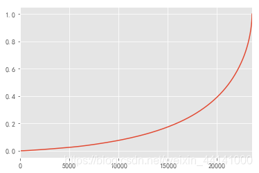
user_cumsum = user_data. sort_values( 'order_amount' ) [ [ 'order_amount' ] ] . cumsum( )
user_cumsum = user_cumsum. apply ( lambda x: x/ user_data[ 'order_amount' ] . sum ( ) )
user_cumsum. head( )
order_amount user_id 10175 0.0 4559 0.0 1948 0.0 925 0.0 10798 0.0
user_cumsum. reset_index( ) [ 'order_amount' ] . plot( )
<matplotlib.axes._subplots.AxesSubplot at 0xab57978>
用户第一次消费时间分布(首购) 用户最后一次消费 新老客消费比
用户分层
用户购买周期(按订单)
用户生命周期(按第一次和最后一次消费时间)
group_user[ 'order_dt' ] . min ( ) . value_counts( ) . plot( )
<matplotlib.axes._subplots.AxesSubplot at 0xcabc7f0>
group_user[ 'order_dt' ] . max ( ) . value_counts( ) . plot( )
<matplotlib.axes._subplots.AxesSubplot at 0xca506a0>
shop_time = group_user[ 'order_dt' ] . agg( [ 'min' , 'max' ] )
shop_time. head( )
min max user_id 1 1997-01-01 1997-01-01 2 1997-01-12 1997-01-12 3 1997-01-02 1998-05-28 4 1997-01-01 1997-12-12 5 1997-01-01 1998-01-03
count = shop_time[ shop_time[ 'min' ] == shop_time[ 'max' ] ]
count. count( )
min    12054
max    12054
dtype: int64
month_user_sum = date. groupby( 'month' ) [ [ 'order_dt' ] ] . count( )
month_user_sum = month_user_sum. cumsum( )
user_class = date. groupby( 'user_id' )
user_min = user_class. month. agg( 'min' ) . reset_index( )
user_min = user_min. groupby( 'month' ) . count( )
user_min
user_id month 1997-01-01 7846 1997-02-01 8476 1997-03-01 7248
new_user = month_user_sum. join( user_min) . fillna( 0 )
new_user
order_dt user_id month 1997-01-01 8928 7846.0 1997-02-01 20200 8476.0 1997-03-01 31798 7248.0 1997-04-01 35579 0.0 1997-05-01 38474 0.0 1997-06-01 41528 0.0 1997-07-01 44470 0.0 1997-08-01 46790 0.0 1997-09-01 49086 0.0 1997-10-01 51648 0.0 1997-11-01 54398 0.0 1997-12-01 56902 0.0 1998-01-01 58934 0.0 1998-02-01 60960 0.0 1998-03-01 63753 0.0 1998-04-01 65631 0.0 1998-05-01 67616 0.0 1998-06-01 69659 0.0
def func_handel ( x) :
return x. user_id / x. order_dt
new_user[ 'proportion' ] = new_user. apply ( func_handel, axis= 1 ) . values
new_user
order_dt user_id proportion month 1997-01-01 8928 7846.0 0.878808 1997-02-01 20200 8476.0 0.419604 1997-03-01 31798 7248.0 0.227939 1997-04-01 35579 0.0 0.000000 1997-05-01 38474 0.0 0.000000 1997-06-01 41528 0.0 0.000000 1997-07-01 44470 0.0 0.000000 1997-08-01 46790 0.0 0.000000 1997-09-01 49086 0.0 0.000000 1997-10-01 51648 0.0 0.000000 1997-11-01 54398 0.0 0.000000 1997-12-01 56902 0.0 0.000000 1998-01-01 58934 0.0 0.000000 1998-02-01 60960 0.0 0.000000 1998-03-01 63753 0.0 0.000000 1998-04-01 65631 0.0 0.000000 1998-05-01 67616 0.0 0.000000 1998-06-01 69659 0.0 0.000000
plt. plot( new_user. index, new_user. proportion)
plt. xticks( rotation= 45 )
plt. show( )
rfm = date. pivot_table( index= 'user_id' , values= [ 'order_products' , 'order_amount' , 'order_dt' ] ,
aggfunc= { 'order_dt' : 'max' , 'order_products' : 'sum' , 'order_amount' : 'sum' } )
rfm. head( )
order_amount order_dt order_products user_id 1 11.77 1997-01-01 1 2 89.00 1997-01-12 6 3 156.46 1998-05-28 16 4 100.50 1997-12-12 7 5 385.61 1998-01-03 29
rfm[ 'R' ] = - ( rfm. order_dt - rfm. order_dt. max ( ) ) / np. timedelta64( 1 , 'D' )
rfm. rename( columns= { 'order_products' : 'F' , 'order_amount' : 'M' } , inplace= True )
rfm. head( )
M order_dt F R user_id 1 11.77 1997-01-01 1 545.0 2 89.00 1997-01-12 6 534.0 3 156.46 1998-05-28 16 33.0 4 100.50 1997-12-12 7 200.0 5 385.61 1998-01-03 29 178.0
def rfm_func ( x) :
level = x. apply ( lambda x: '1' if x>= 0 else '0' )
label = level. R + level. F + level. M
d = {
'111' : '重要客户' ,
'011' : '重要保持客户' ,
'101' : '重要挽留客户' ,
'001' : '重要发展客户' ,
'110' : '一般客户' ,
'010' : '一般保持客户' ,
'100' : '一般挽留客户' ,
'000' : '一般发展客户'
}
result = d[ label]
return result
rfm[ 'label' ] = rfm[ [ 'R' , 'F' , 'M' ] ] . apply ( lambda x: x- x. mean( ) ) . apply ( rfm_func, axis= 1 )
rfm. head( )
M order_dt F R label user_id 1 11.77 1997-01-01 1 545.0 一般挽留客户 2 89.00 1997-01-12 6 534.0 一般挽留客户 3 156.46 1998-05-28 16 33.0 重要保持客户 4 100.50 1997-12-12 7 200.0 一般发展客户 5 385.61 1998-01-03 29 178.0 重要保持客户
rfm. groupby( 'label' ) . sum ( )
M F R label 一般保持客户 19937.45 1712 29448.0 一般发展客户 196971.23 13977 591108.0 一般客户 7181.28 650 36295.0 一般挽留客户 438291.81 29346 6951815.0 重要保持客户 1592039.62 107789 517267.0 重要发展客户 45785.01 2023 56636.0 重要客户 167080.83 11121 358363.0 重要挽留客户 33028.40 1263 114482.0
rfm. loc[ rfm. label == '重要客户' , 'color' ] = 'g'
rfm. loc[ ~ ( rfm. label == '重要客户' ) , 'color' ] = 'r'
rfm. plot. scatter( 'F' , 'R' , c= rfm. color)
<matplotlib.axes._subplots.AxesSubplot at 0xca0f908>
尽量用小部分的用户涵盖大部分的额度 不要为了数据好看划分等级
pivot_counts = date. pivot_table( index= 'user_id' , columns= 'month' , values= 'order_dt' , aggfunc= 'count' ) . fillna( 0 )
pivot_counts. head( )
month 1997-01-01 00:00:00 1997-02-01 00:00:00 1997-03-01 00:00:00 1997-04-01 00:00:00 1997-05-01 00:00:00 1997-06-01 00:00:00 1997-07-01 00:00:00 1997-08-01 00:00:00 1997-09-01 00:00:00 1997-10-01 00:00:00 1997-11-01 00:00:00 1997-12-01 00:00:00 1998-01-01 00:00:00 1998-02-01 00:00:00 1998-03-01 00:00:00 1998-04-01 00:00:00 1998-05-01 00:00:00 1998-06-01 00:00:00 user_id 1 1.0 0.0 0.0 0.0 0.0 0.0 0.0 0.0 0.0 0.0 0.0 0.0 0.0 0.0 0.0 0.0 0.0 0.0 2 2.0 0.0 0.0 0.0 0.0 0.0 0.0 0.0 0.0 0.0 0.0 0.0 0.0 0.0 0.0 0.0 0.0 0.0 3 1.0 0.0 1.0 1.0 0.0 0.0 0.0 0.0 0.0 0.0 2.0 0.0 0.0 0.0 0.0 0.0 1.0 0.0 4 2.0 0.0 0.0 0.0 0.0 0.0 0.0 1.0 0.0 0.0 0.0 1.0 0.0 0.0 0.0 0.0 0.0 0.0 5 2.0 1.0 0.0 1.0 1.0 1.0 1.0 0.0 1.0 0.0 0.0 2.0 1.0 0.0 0.0 0.0 0.0 0.0
purchase_user = pivot_counts. applymap( lambda x: 1 if x> 0 else 0 )
purchase_user. tail( )
month 1997-01-01 00:00:00 1997-02-01 00:00:00 1997-03-01 00:00:00 1997-04-01 00:00:00 1997-05-01 00:00:00 1997-06-01 00:00:00 1997-07-01 00:00:00 1997-08-01 00:00:00 1997-09-01 00:00:00 1997-10-01 00:00:00 1997-11-01 00:00:00 1997-12-01 00:00:00 1998-01-01 00:00:00 1998-02-01 00:00:00 1998-03-01 00:00:00 1998-04-01 00:00:00 1998-05-01 00:00:00 1998-06-01 00:00:00 user_id 23566 0 0 1 0 0 0 0 0 0 0 0 0 0 0 0 0 0 0 23567 0 0 1 0 0 0 0 0 0 0 0 0 0 0 0 0 0 0 23568 0 0 1 1 0 0 0 0 0 0 0 0 0 0 0 0 0 0 23569 0 0 1 0 0 0 0 0 0 0 0 0 0 0 0 0 0 0 23570 0 0 1 0 0 0 0 0 0 0 0 0 0 0 0 0 0 0
def active_status ( data) :
status = [ ]
for i in range ( 18 ) :
if data[ i] == 0 :
if len ( status) == 0 :
status. append( 'unregister' )
else :
if status[ i- 1 ] == 'unregister' :
status. append( 'unregister' )
else :
status. append( 'unactive' )
else :
if len ( status) == 0 :
status. append( 'new' )
else :
if status[ i- 1 ] == 'unregister' :
status. append( 'new' )
elif status[ i- 1 ] == 'unactive' :
status. append( 'return' )
else :
status. append( 'active' )
return status
purchase_user = purchase_user. apply ( active_status, axis= 1 )
purchase_user. tail( )
month 1997-01-01 00:00:00 1997-02-01 00:00:00 1997-03-01 00:00:00 1997-04-01 00:00:00 1997-05-01 00:00:00 1997-06-01 00:00:00 1997-07-01 00:00:00 1997-08-01 00:00:00 1997-09-01 00:00:00 1997-10-01 00:00:00 1997-11-01 00:00:00 1997-12-01 00:00:00 1998-01-01 00:00:00 1998-02-01 00:00:00 1998-03-01 00:00:00 1998-04-01 00:00:00 1998-05-01 00:00:00 1998-06-01 00:00:00 user_id 23566 unregister unregister new unactive unactive unactive unactive unactive unactive unactive unactive unactive unactive unactive unactive unactive unactive unactive 23567 unregister unregister new unactive unactive unactive unactive unactive unactive unactive unactive unactive unactive unactive unactive unactive unactive unactive 23568 unregister unregister new active unactive unactive unactive unactive unactive unactive unactive unactive unactive unactive unactive unactive unactive unactive 23569 unregister unregister new unactive unactive unactive unactive unactive unactive unactive unactive unactive unactive unactive unactive unactive unactive unactive 23570 unregister unregister new unactive unactive unactive unactive unactive unactive unactive unactive unactive unactive unactive unactive unactive unactive unactive
purchase_user_status = purchase_user. replace( 'unregister' , np. NaN) . apply ( lambda x: pd. value_counts( x) )
purchase_user_status
month 1997-01-01 00:00:00 1997-02-01 00:00:00 1997-03-01 00:00:00 1997-04-01 00:00:00 1997-05-01 00:00:00 1997-06-01 00:00:00 1997-07-01 00:00:00 1997-08-01 00:00:00 1997-09-01 00:00:00 1997-10-01 00:00:00 1997-11-01 00:00:00 1997-12-01 00:00:00 1998-01-01 00:00:00 1998-02-01 00:00:00 1998-03-01 00:00:00 1998-04-01 00:00:00 1998-05-01 00:00:00 1998-06-01 00:00:00 active NaN 1157.0 1681 1773.0 852.0 747.0 746.0 604.0 528.0 532.0 624.0 632.0 512.0 472.0 571.0 518.0 459.0 446.0 new 7846.0 8476.0 7248 NaN NaN NaN NaN NaN NaN NaN NaN NaN NaN NaN NaN NaN NaN NaN return NaN NaN 595 1049.0 1362.0 1592.0 1434.0 1168.0 1211.0 1307.0 1404.0 1232.0 1025.0 1079.0 1489.0 919.0 1029.0 1060.0 unactive NaN 6689.0 14046 20748.0 21356.0 21231.0 21390.0 21798.0 21831.0 21731.0 21542.0 21706.0 22033.0 22019.0 21510.0 22133.0 22082.0 22064.0
purchase_user_status. fillna( 0 ) . T
active new return unactive month 1997-01-01 0.0 7846.0 0.0 0.0 1997-02-01 1157.0 8476.0 0.0 6689.0 1997-03-01 1681.0 7248.0 595.0 14046.0 1997-04-01 1773.0 0.0 1049.0 20748.0 1997-05-01 852.0 0.0 1362.0 21356.0 1997-06-01 747.0 0.0 1592.0 21231.0 1997-07-01 746.0 0.0 1434.0 21390.0 1997-08-01 604.0 0.0 1168.0 21798.0 1997-09-01 528.0 0.0 1211.0 21831.0 1997-10-01 532.0 0.0 1307.0 21731.0 1997-11-01 624.0 0.0 1404.0 21542.0 1997-12-01 632.0 0.0 1232.0 21706.0 1998-01-01 512.0 0.0 1025.0 22033.0 1998-02-01 472.0 0.0 1079.0 22019.0 1998-03-01 571.0 0.0 1489.0 21510.0 1998-04-01 518.0 0.0 919.0 22133.0 1998-05-01 459.0 0.0 1029.0 22082.0 1998-06-01 446.0 0.0 1060.0 22064.0
purchase_user_status. fillna( 0 ) . T. plot. area( )
<matplotlib.axes._subplots.AxesSubplot at 0xc9fc0b8>
purchase_user_status. fillna( 0 ) . T. apply ( lambda x: x/ x. sum ( ) , axis= 1 )
active new return unactive month 1997-01-01 0.000000 1.000000 0.000000 0.000000 1997-02-01 0.070886 0.519299 0.000000 0.409815 1997-03-01 0.071319 0.307510 0.025244 0.595927 1997-04-01 0.075223 0.000000 0.044506 0.880272 1997-05-01 0.036148 0.000000 0.057785 0.906067 1997-06-01 0.031693 0.000000 0.067543 0.900764 1997-07-01 0.031650 0.000000 0.060840 0.907510 1997-08-01 0.025626 0.000000 0.049555 0.924820 1997-09-01 0.022401 0.000000 0.051379 0.926220 1997-10-01 0.022571 0.000000 0.055452 0.921977 1997-11-01 0.026474 0.000000 0.059567 0.913958 1997-12-01 0.026814 0.000000 0.052270 0.920916 1998-01-01 0.021723 0.000000 0.043487 0.934790 1998-02-01 0.020025 0.000000 0.045779 0.934196 1998-03-01 0.024226 0.000000 0.063174 0.912601 1998-04-01 0.021977 0.000000 0.038990 0.939033 1998-05-01 0.019474 0.000000 0.043657 0.936869 1998-06-01 0.018922 0.000000 0.044972 0.936105
回流用户:之前没消费,本月才消费(唤回运营) 活跃用户:持续消费(消费运营的质量) 不活跃用户:流失用户
order_diff = group_user. apply ( lambda x: ( x. order_dt - x. order_dt. shift( ) ) / np. timedelta64( 1 , 'D' ) )
order_diff. hist( bins= 20 )
<matplotlib.axes._subplots.AxesSubplot at 0x1299db00>
user_period = group_user. order_dt. agg( [ 'max' , 'min' ] )
user_period = user_period. apply ( lambda x: ( x[ 'max' ] - x[ 'min' ] ) / np. timedelta64( 1 , 'D' ) , axis= 1 )
user_period. describe( )
count    23570.000000
mean       134.871956
std        180.574109
min          0.000000
25%          0.000000
50%          0.000000
75%        294.000000
max        544.000000
dtype: float64
user_period = pd. DataFrame( user_period, columns= [ 'diff' ] )
user_period. head( )
diff user_id 1 0.0 2 0.0 3 511.0 4 345.0 5 367.0
user_period[ user_period[ 'diff' ] != 0 ] . hist( bins= 40 )
array([[<matplotlib.axes._subplots.AxesSubplot object at 0x000000000B3A2DD8>]], dtype=object)
pivot_counts. head( 10 )
month 1997-01-01 00:00:00 1997-02-01 00:00:00 1997-03-01 00:00:00 1997-04-01 00:00:00 1997-05-01 00:00:00 1997-06-01 00:00:00 1997-07-01 00:00:00 1997-08-01 00:00:00 1997-09-01 00:00:00 1997-10-01 00:00:00 1997-11-01 00:00:00 1997-12-01 00:00:00 1998-01-01 00:00:00 1998-02-01 00:00:00 1998-03-01 00:00:00 1998-04-01 00:00:00 1998-05-01 00:00:00 1998-06-01 00:00:00 user_id 1 1.0 0.0 0.0 0.0 0.0 0.0 0.0 0.0 0.0 0.0 0.0 0.0 0.0 0.0 0.0 0.0 0.0 0.0 2 2.0 0.0 0.0 0.0 0.0 0.0 0.0 0.0 0.0 0.0 0.0 0.0 0.0 0.0 0.0 0.0 0.0 0.0 3 1.0 0.0 1.0 1.0 0.0 0.0 0.0 0.0 0.0 0.0 2.0 0.0 0.0 0.0 0.0 0.0 1.0 0.0 4 2.0 0.0 0.0 0.0 0.0 0.0 0.0 1.0 0.0 0.0 0.0 1.0 0.0 0.0 0.0 0.0 0.0 0.0 5 2.0 1.0 0.0 1.0 1.0 1.0 1.0 0.0 1.0 0.0 0.0 2.0 1.0 0.0 0.0 0.0 0.0 0.0 6 1.0 0.0 0.0 0.0 0.0 0.0 0.0 0.0 0.0 0.0 0.0 0.0 0.0 0.0 0.0 0.0 0.0 0.0 7 1.0 0.0 0.0 0.0 0.0 0.0 0.0 0.0 0.0 1.0 0.0 0.0 0.0 0.0 1.0 0.0 0.0 0.0 8 1.0 1.0 0.0 0.0 0.0 1.0 1.0 0.0 0.0 0.0 2.0 1.0 0.0 0.0 1.0 0.0 0.0 0.0 9 1.0 0.0 0.0 0.0 1.0 0.0 0.0 0.0 0.0 0.0 0.0 0.0 0.0 0.0 0.0 0.0 0.0 1.0 10 1.0 0.0 0.0 0.0 0.0 0.0 0.0 0.0 0.0 0.0 0.0 0.0 0.0 0.0 0.0 0.0 0.0 0.0
re_purchase = pivot_counts. applymap( lambda x: 1 if x> 1 else np. NaN if x== 0 else 0 )
re_purchase. head( 10 )
month 1997-01-01 00:00:00 1997-02-01 00:00:00 1997-03-01 00:00:00 1997-04-01 00:00:00 1997-05-01 00:00:00 1997-06-01 00:00:00 1997-07-01 00:00:00 1997-08-01 00:00:00 1997-09-01 00:00:00 1997-10-01 00:00:00 1997-11-01 00:00:00 1997-12-01 00:00:00 1998-01-01 00:00:00 1998-02-01 00:00:00 1998-03-01 00:00:00 1998-04-01 00:00:00 1998-05-01 00:00:00 1998-06-01 00:00:00 user_id 1 0.0 NaN NaN NaN NaN NaN NaN NaN NaN NaN NaN NaN NaN NaN NaN NaN NaN NaN 2 1.0 NaN NaN NaN NaN NaN NaN NaN NaN NaN NaN NaN NaN NaN NaN NaN NaN NaN 3 0.0 NaN 0.0 0.0 NaN NaN NaN NaN NaN NaN 1.0 NaN NaN NaN NaN NaN 0.0 NaN 4 1.0 NaN NaN NaN NaN NaN NaN 0.0 NaN NaN NaN 0.0 NaN NaN NaN NaN NaN NaN 5 1.0 0.0 NaN 0.0 0.0 0.0 0.0 NaN 0.0 NaN NaN 1.0 0.0 NaN NaN NaN NaN NaN 6 0.0 NaN NaN NaN NaN NaN NaN NaN NaN NaN NaN NaN NaN NaN NaN NaN NaN NaN 7 0.0 NaN NaN NaN NaN NaN NaN NaN NaN 0.0 NaN NaN NaN NaN 0.0 NaN NaN NaN 8 0.0 0.0 NaN NaN NaN 0.0 0.0 NaN NaN NaN 1.0 0.0 NaN NaN 0.0 NaN NaN NaN 9 0.0 NaN NaN NaN 0.0 NaN NaN NaN NaN NaN NaN NaN NaN NaN NaN NaN NaN 0.0 10 0.0 NaN NaN NaN NaN NaN NaN NaN NaN NaN NaN NaN NaN NaN NaN NaN NaN NaN
re_purchase. apply ( lambda x: x. sum ( ) / x. count( ) ) . plot( figsize= ( 10 , 4 ) )
<matplotlib.axes._subplots.AxesSubplot at 0x28a1390>
repurchase = pivot_counts. applymap( lambda x: 1 if x> 0 else 0 )
repurchase. head( 10 )
month 1997-01-01 00:00:00 1997-02-01 00:00:00 1997-03-01 00:00:00 1997-04-01 00:00:00 1997-05-01 00:00:00 1997-06-01 00:00:00 1997-07-01 00:00:00 1997-08-01 00:00:00 1997-09-01 00:00:00 1997-10-01 00:00:00 1997-11-01 00:00:00 1997-12-01 00:00:00 1998-01-01 00:00:00 1998-02-01 00:00:00 1998-03-01 00:00:00 1998-04-01 00:00:00 1998-05-01 00:00:00 1998-06-01 00:00:00 user_id 1 1 0 0 0 0 0 0 0 0 0 0 0 0 0 0 0 0 0 2 1 0 0 0 0 0 0 0 0 0 0 0 0 0 0 0 0 0 3 1 0 1 1 0 0 0 0 0 0 1 0 0 0 0 0 1 0 4 1 0 0 0 0 0 0 1 0 0 0 1 0 0 0 0 0 0 5 1 1 0 1 1 1 1 0 1 0 0 1 1 0 0 0 0 0 6 1 0 0 0 0 0 0 0 0 0 0 0 0 0 0 0 0 0 7 1 0 0 0 0 0 0 0 0 1 0 0 0 0 1 0 0 0 8 1 1 0 0 0 1 1 0 0 0 1 1 0 0 1 0 0 0 9 1 0 0 0 1 0 0 0 0 0 0 0 0 0 0 0 0 1 10 1 0 0 0 0 0 0 0 0 0 0 0 0 0 0 0 0 0
def Repurchase ( data) :
is_purchase = [ ]
for i in range ( 0 , 17 ) :
if data[ i] > 0 :
if data[ i+ 1 ] > 0 :
is_purchase. append( 1 )
else :
is_purchase. append( 0 )
else :
is_purchase. append( np. NaN)
is_purchase. append( np. NaN)
return is_purchase
repurchase = repurchase. apply ( Repurchase, axis= 1 )
repurchase. head( 5 )
month 1997-01-01 00:00:00 1997-02-01 00:00:00 1997-03-01 00:00:00 1997-04-01 00:00:00 1997-05-01 00:00:00 1997-06-01 00:00:00 1997-07-01 00:00:00 1997-08-01 00:00:00 1997-09-01 00:00:00 1997-10-01 00:00:00 1997-11-01 00:00:00 1997-12-01 00:00:00 1998-01-01 00:00:00 1998-02-01 00:00:00 1998-03-01 00:00:00 1998-04-01 00:00:00 1998-05-01 00:00:00 1998-06-01 00:00:00 user_id 1 0.0 NaN NaN NaN NaN NaN NaN NaN NaN NaN NaN NaN NaN NaN NaN NaN NaN NaN 2 0.0 NaN NaN NaN NaN NaN NaN NaN NaN NaN NaN NaN NaN NaN NaN NaN NaN NaN 3 0.0 NaN 1.0 0.0 NaN NaN NaN NaN NaN NaN 0.0 NaN NaN NaN NaN NaN 0.0 NaN 4 0.0 NaN NaN NaN NaN NaN NaN 0.0 NaN NaN NaN 0.0 NaN NaN NaN NaN NaN NaN 5 1.0 0.0 NaN 1.0 1.0 1.0 0.0 NaN 0.0 NaN NaN 1.0 0.0 NaN NaN NaN NaN NaN
repurchase. apply ( lambda x: x. sum ( ) / x. count( ) ) . plot( figsize= ( 10 , 4 ) )
D:\Anaconda3\lib\site-packages\ipykernel_launcher.py:1: RuntimeWarning: invalid value encountered in true_divide
  """Entry point for launching an IPython kernel.


<matplotlib.axes._subplots.AxesSubplot at 0xaad40b8>


 1506
1506


 被折叠的 条评论
为什么被折叠?
被折叠的 条评论
为什么被折叠?
 到【灌水乐园】发言


