Python | 海表面温度(SST) | 长期趋势和异常分析

趋势和异常分析（Trend and anomaly)在大气和海洋学研究中被广泛用于探测长期变化。

趋势分析（Trend Analysis）：

趋势分析是一种用于检测数据随时间的变化趋势的方法。在海洋学和大气学中，常见的趋势分析包括海表面温度（SST）、海平面上升、气温变化等。趋势分析通常包括以下步骤：

• 数据预处理：首先需要对数据进行预处理，包括去除季节循环、填补缺失值等。
• 计算趋势：采用统计方法（如线性回归、非线性回归）来计算数据随时间的变化趋势。常见的趋势计算方法包括最小二乘法、曲线拟合等。
• 趋势显著性检验：对计算得到的趋势进行显著性检验，以确定趋势是否具有统计显著性。常见的显著性检验方法包括t检验、F检验等。
• 趋势可视化：将计算得到的趋势以图形方式呈现，通常使用折线图或柱状图来展示数据随时间的变化趋势。

趋势分析的结果可以帮助科学家们了解气候系统的长期演变趋势，从而预测未来可能的变化情况。

异常分析（Anomaly Analysis）：

异常分析是一种用于检测数据中非正常事件或突发事件的方法。在海洋学和大气学中，异常分析通常用于检测气候系统中的异常事件，如El Niño事件、极端气候事件等。异常分析通常包括以下步骤：

• 基准确定：选择一个合适的基准期，通常是一段相对稳定的时间段，用于计算异常值。
• 计算异常：将观测数据与基准期的平均值进行比较，计算出每个时间点的异常值。异常值表示该时间点的数据与基准期相比的偏离程度。
• 异常检测：对计算得到的异常值进行检测，识别出突发事件或非正常事件。
• 异常可视化：将计算得到的异常值以图形方式呈现，通常使用折线图或柱状图来展示异常事件的发生情况。
  异常分析的结果可以帮助科学家们理解气候系统中的非正常事件，从而采取相应的应对措施或预测未来可能发生的异常情况。

---

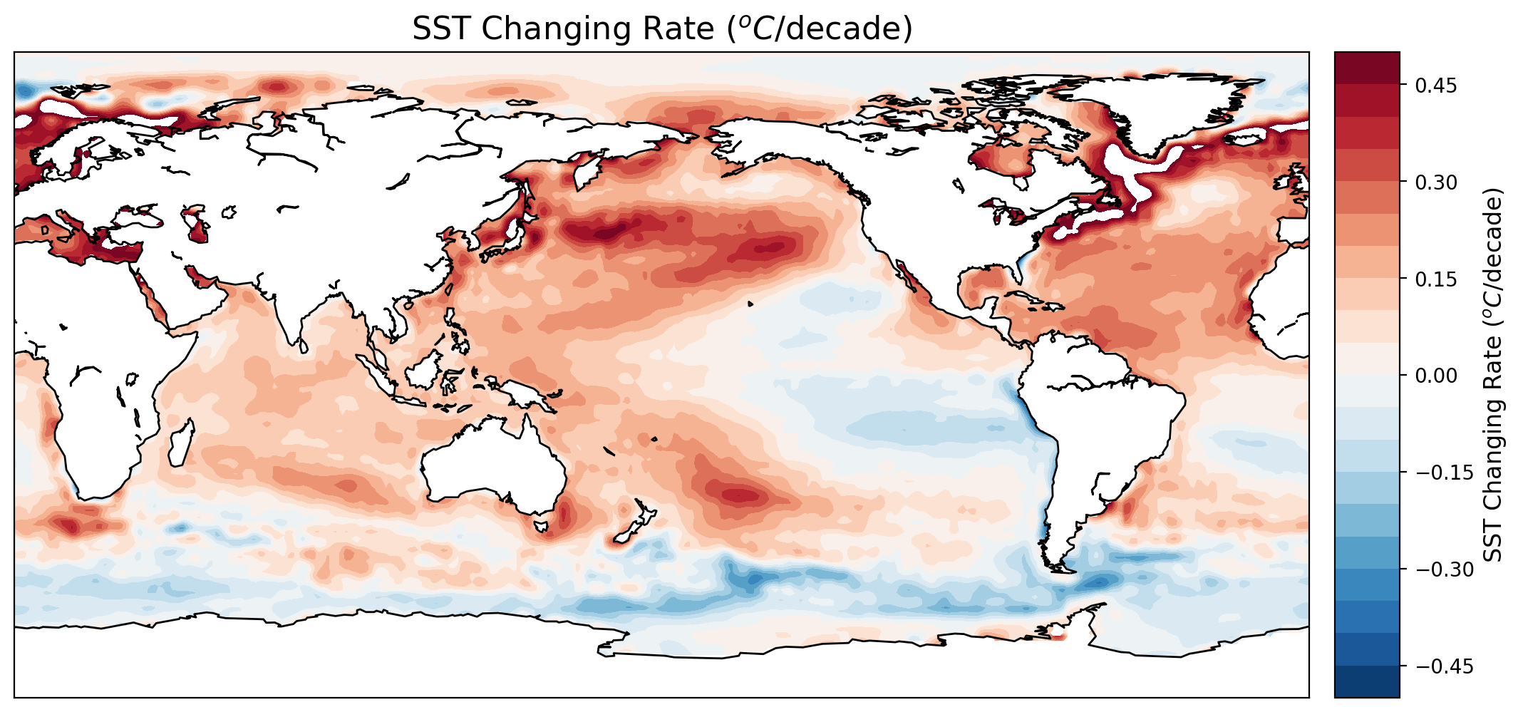
本案例分析以海表温度为例，计算了1982年至2016年全球每十年的温度变化率。此外，还给出了其面积加权的全球月海温异常时间序列。

• 数据来源：
  NOAA Optimum Interpolation (OI) Sea Surface Temperature (SST) V2

• 下载地址：
  https://www.esrl.noaa.gov/psd/data/gridded/data.noaa.oisst.v2.html

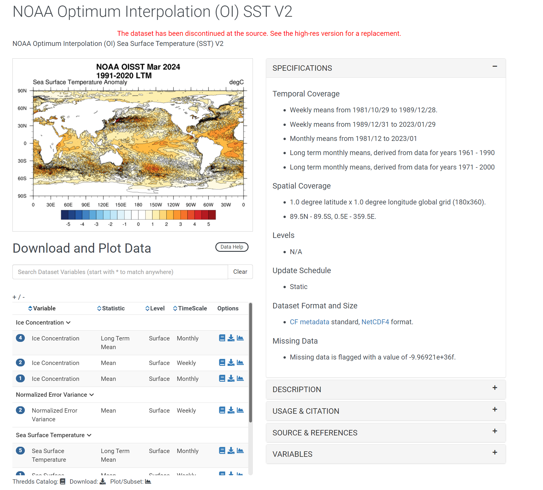
NOAA Optimum Interpolation (OI) Sea Surface Temperature (SST) V2

• 空间分辨率:

1.0纬度 x 1.0经度全球网格(180x360)。

• 覆盖范围

89.5 N-89.5 S 

0.5 E-359.5 E.

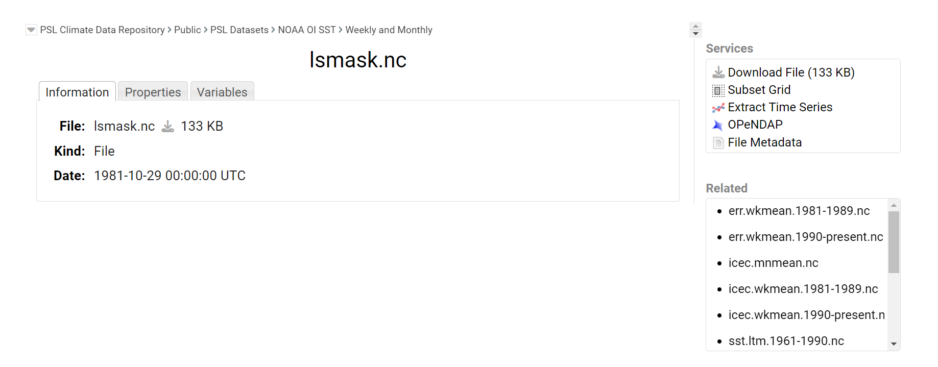
因为oisst是一个插值数据，所以它覆盖了海洋和陆地。
因此，必须同时使用陆地-海洋掩膜数据，可以从如下网站获得：

https://psl.noaa.gov/repository/entry/show?entryid=b5492d1c-7d9c-47f7-b058-e84030622bbd

1. 加载基础库

import numpy as np
import datetime 
import cftime
from netCDF4 import Dataset as netcdf # netcdf4-python module
import netCDF4 as nc
import matplotlib.pyplot as plt
from mpl_toolkits.basemap import Basemap
import matplotlib.dates as mdates
from matplotlib.dates import MonthLocator, WeekdayLocator, DateFormatter
import matplotlib.ticker as ticker
from matplotlib.pylab import rcParams
rcParams['figure.figsize'] = 15, 6
import warnings
warnings.simplefilter('ignore')

# Your code continues here

# ================================================================================================
# Author: %(Jianpu)s | Affiliation: Hohai
# Email : %(email)s
# Last modified: 2024-04-04 12:28:06
# Filename: Trend and Anomaly Analyses.py
# Description:
# =================================================================================================

2. 读取数据、提取变量

2.1 Read SST

ncset= netcdf(r'G:/code_daily/sst.mnmean.nc')
lons = ncset['lon'][:]  
lats = ncset['lat'][:]           
sst  = ncset['sst'][1:421,:,:]    # 1982-2016 to make it divisible by 12
nctime = ncset['time'][1:421]
t_unit = ncset['time'].units

try :
    t_cal =ncset['time'].calendar
except AttributeError : # Attribute doesn't exist
    t_cal = u"gregorian" # or standard

nt, nlat, nlon = sst.shape
ngrd = nlon*nlat

2.2 解析时间

datevar = nc.num2date(nctime,units = "days since 1800-1-1 00:00:00")
print(datevar.shape)

datevar[0:5]

2.3读取 mask (1=ocen, 0=land)

lmfile = 'G:/code_daily/lsmask.nc'
lmset  = netcdf(lmfile)
lsmask = lmset['mask'][0,:,:]
lsmask = lsmask-1

num_repeats = nt
lsm = np.stack([lsmask]*num_repeats,axis=-1).transpose((2,0,1))
lsm.shape

2.3 将海温的陆地区域进行掩膜

sst = np.ma.masked_array(sst, mask=lsm)
3. Trend Analysis
3.1 计算线性趋势
sst_grd  = sst.reshape((nt, ngrd), order='F') 
x        = np.linspace(1,nt,nt)#.reshape((nt,1))
sst_rate = np.empty((ngrd,1))
sst_rate[:,:] = np.nan

for i in range(ngrd): 
    y = sst_grd[:,i]   
    if(not np.ma.is_masked(y)):         
        z = np.polyfit(x, y, 1)
        sst_rate[i,0] = z[0]*120.0
        #slope, intercept, r_value, p_value, std_err = stats.linregress(x, sst_grd[:,i])
        #sst_rate[i,0] = slope*120.0     
    
sst_rate = sst_rate.reshape((nlat,nlon), order='F')

3 绘制趋势空间分布

plt.figure(dpi=200)
m = Basemap(projection='cyl', llcrnrlon=min(lons), llcrnrlat=min(lats),
        urcrnrlon=max(lons), urcrnrlat=max(lats))

x, y = m(*np.meshgrid(lons, lats))
clevs = np.linspace(-0.5, 0.5, 21)
cs = m.contourf(x, y, sst_rate.squeeze(), clevs, cmap=plt.cm.RdBu_r)
m.drawcoastlines()
#m.fillcontinents(color='#000000',lake_color='#99ffff')

cb = m.colorbar(cs)
cb.set_label('SST Changing Rate ($^oC$/decade)', fontsize=12)
plt.title('SST Changing Rate ($^oC$/decade)', fontsize=16)

4. Anomaly analysis

4.1 转换数据大小为： (nyear) x (12) x (lat x lon)

sst_grd_ym  = sst.reshape((12,round(nt/12), ngrd), order='F').transpose((1,0,2))
sst_grd_ym.shape

4.2 计算季节趋势

sst_grd_clm = np.mean(sst_grd_ym, axis=0)
sst_grd_clm.shape

4.3 去除季节趋势

sst_grd_anom = (sst_grd_ym - sst_grd_clm).transpose((1,0,2)).reshape((nt, nlat, nlon), order='F')
sst_grd_anom.shape

4.4 计算区域权重

4.4.1 确认经纬度的方向

print(lats[0:12])
print(lons[0:12])

4.4.2 计算随纬度变化的区域权重

lonx, latx = np.meshgrid(lons, lats)
weights = np.cos(latx * np.pi / 180.)
print(weights.shape)

4.4.3 计算全球、北半球、南半球的有效网格总面积

sst_glb_avg = np.zeros(nt)
sst_nh_avg  = np.zeros(nt)
sst_sh_avg  = np.zeros(nt)

for it in np.arange(nt):
    sst_glb_avg[it] = np.ma.average(sst_grd_anom[it, :], weights=weights)
    sst_nh_avg[it]  = np.ma.average(sst_grd_anom[it,0:round(nlat/2),:],    weights=weights[0:round(nlat/2),:])
    sst_sh_avg[it]  = np.ma.average(sst_grd_anom[it,round(nlat/2):nlat,:], weights=weights[round(nlat/2):nlat,:])

4.5 转换时间为字符串格式

datestr = [date.strftime('%Y-%m-%d') for date in datevar]

5. 绘制海温异常时间序列

fig, ax = plt.subplots(1, 1 , figsize=(15,5),dpi=200)

ax.plot(datestr[::12], sst_glb_avg[::12], color='b', linewidth=2, label='GLB')
ax.plot(datestr[::12], sst_nh_avg[::12],  color='r', linewidth=2, label='NH')
ax.plot(datestr[::12], sst_sh_avg[::12],  color='g', linewidth=2, label='SH')
ax.set_xticklabels(datestr[::12], rotation=45)
ax.axhline(0, linewidth=1, color='k')
ax.legend()
ax.set_title('Monthly SST Anomaly Time Series (1982 - 2016)', fontsize=16)
ax.set_xlabel('Month/Year ', fontsize=12)
ax.set_ylabel('$^oC$', fontsize=12)
ax.set_ylim(-0.6, 0.6)
fig.set_figheight(9)

# rotate and align the tick labels so they look better
fig.autofmt_xdate()
# use a more precise date string for the x axis locations in the toolbar
ax.fmt_xdata = mdates.DateFormatter('%Y')

http://unidata.github.io/netcdf4-python/

http://www.scipy.org/
​

本文由mdnice多平台发布