Python | 计算位涡平流项

写在前面

最近忙着复习、考试…都没怎么空敲代码，还得再准备一周考试。。。等考完试再慢慢更新了，今天先来浅更一个简单但是使用的python code

---

• 在做动力机制分析时，我们常常需要借助收支方程来诊断不同过程的贡献，其中最常见的一项就包括水平平流项，如下所示，其中var表示某一个变量，V表示水平风场。

$$-V\cdot \nabla var$$

以位涡的水平平流项为例，展开为

$$-(u\frac{\partial pv}{\partial x}+v\frac{\partial pv}{\partial y})$$

其物理解释为：

• 位涡受背景气流的调控作用。在存在背景气流的情况下，这个位涡信号受到多少平流的贡献

对于这种诊断量的计算，平流项，散度项，都可以通过metpy来计算。之前介绍过一次，因为metpy为大大简便了计算

但是，如果这样还是不放心应该怎么办呢，这里可以基于numpy的方式自己来手动计算平流项，然后比较两种方法的差异。下面我就从两种计算方式以及检验方式来计算pv的水平平流项

首先来导入基本的库和数据，我这里用的wrf输出的风场以及位涡pv,同时，为了减少计算量，对于数据进行区域和高度层的截取

• 经纬度可以直接从nc数据中获取，我下面是之前的代码直接拿过来用了，还是以wrf*out数据来提取的lon&lat

import numpy as np
import pandas as pd
import xarray as xr
import matplotlib.pyplot as plt
import cartopy.crs as ccrs
import glob
from matplotlib.colors import ListedColormap 
from wrf import getvar,pvo,interplevel,destagger,latlon_coords
from cartopy.mpl.ticker import LongitudeFormatter,LatitudeFormatter
from netCDF4 import Dataset
import matplotlib as mpl   
from metpy.units import units
import metpy.constants as constants
import metpy.calc as mpcalc
import cmaps
# units.define('PVU = 1e-6 m^2 s^-1 K kg^-1 = pvu')
import cartopy.feature as cfeature
f_w   = r'L:\JAS\wind.nc'
f_pv  = r'L:\JAS\pv.nc'
def  cal_dxdy(file):
    ncfile = Dataset(file)
    P = getvar(ncfile, "pressure")
    lats, lons = latlon_coords(P)
    lon = lons[0]
    lon[lon<=0]=lon[lon<=0]+360
    lat = lats[:,0]
    dx, dy = mpcalc.lat_lon_grid_deltas(lon.data, lat.data)
    return lon,lat,dx,dy
path  = r'L:\\wrf*'
filelist = glob.glob(path)
filelist.sort()
lon,lat,_,_ = cal_dxdy(filelist[-1]) 
dw = xr.open_dataset(f_w).sel(level=850,lat=slice(0,20),lon=slice(100,150))
dp = xr.open_dataset(f_pv).sel(level=850,lat=slice(0,20),lon=slice(100,150))
u = dw.u.sel(lat=slice(0,20),lon=slice(100,150))
v = dw.v.sel(lat=slice(0,20),lon=slice(100,150))
pv = dp.pv.sel(lat=slice(0,20),lon=slice(100,150))
lon = u.lon
lat = u.lat

metpy

###############################################################################
#####                  
#####                      using metpy to calculate advection
#####
###############################################################################
tadv = mpcalc.advection(pv*units('pvu'), u*units('m/s'), v*units('m/s'))
print(tadv)
###############################################################################
#####                  
#####                       plot advection
#####
###############################################################################
# start figure and set axis
fig, (ax) = plt.subplots(1, 1, figsize=(8, 6),dpi=200, subplot_kw={'projection': ccrs.PlateCarree()})
proj = ccrs.PlateCarree()
# plot isotherms
cs = ax.contour(lon, lat, pv[-1]*10**4, 8, 
            colors='k',
              linewidths=0.2)
ax.coastlines('10m',linewidths=0.5,facecolor='w',edgecolor='k')
box = [100,121,0,20]
ax.set_extent(box,crs=ccrs.PlateCarree())
ax.set_xticks(np.arange(box[0],box[1], 10), crs=proj)
ax.set_yticks(np.arange(box[2], box[3], 5), crs=proj)
ax.xaxis.set_major_formatter(LongitudeFormatter())
ax.yaxis.set_major_formatter(LatitudeFormatter())
# plot tmperature advection and convert units to Kelvin per 3 hours
cf = ax.contourf(lon, lat,   tadv[10]*10**4, 
                 np.linspace(-4, 4, 21), extend='both',
                 cmap='RdYlGn', alpha=0.75)
plt.colorbar(cf, pad=0.05, aspect=20,shrink=0.75)
ax.set_title('PV Advection Calculation')
plt.show()

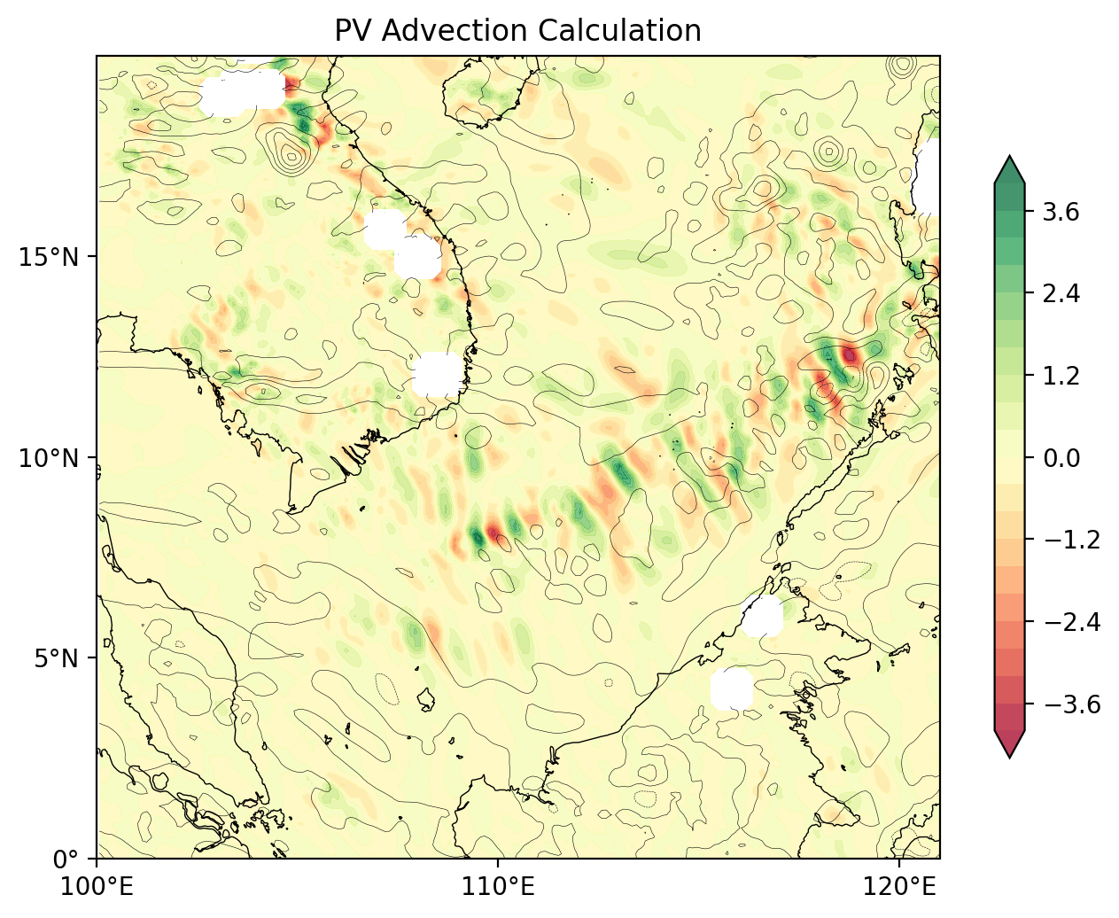
metpy官网也提供了计算示例：

• https://unidata.github.io/MetPy/latest/examples/calculations/Advection.html

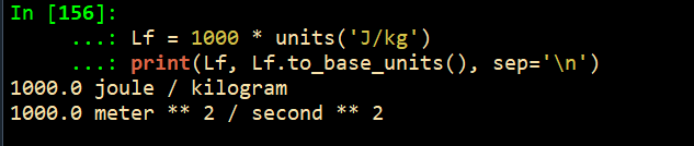
当然，这里需要提醒的是，在使用metpy计算时，最好是将变量带上单位，这样可以保证计算结果的量级没有问题；或者最后将其转换为国际基本单位:m , s ,g ...

关于metpt中单位unit的使用，可以在官网进行查阅：

• https://unidata.github.io/MetPy/latest/tutorials/unit_tutorial.html

Lf = 1000 * units('J/kg')
print(Lf, Lf.to_base_units(), sep='\n')

1000.0 joule / kilogram
1000.0 meter ** 2 / second ** 2

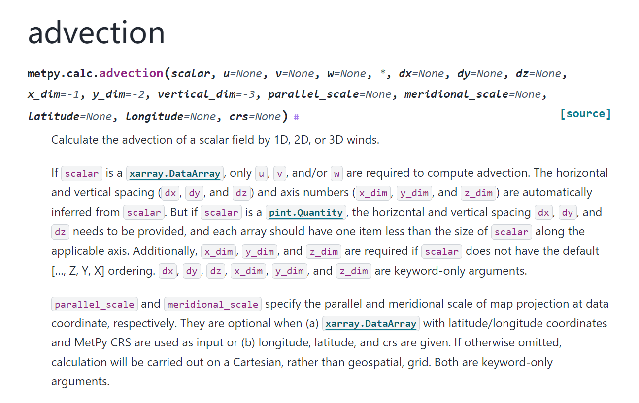
当然，还可以点击 source code 去了解这个函数背后的计算过程：

• https://github.com/Unidata/MetPy/blob/v1.6.2/src/metpy/calc/kinematics.py#L359-L468

def advection(
    scalar,
    u=None,
    v=None,
    w=None,
    *,
    dx=None,
    dy=None,
    dz=None,
    x_dim=-1,
    y_dim=-2,
    vertical_dim=-3,
    parallel_scale=None,
    meridional_scale=None
):
    r"""Calculate the advection of a scalar field by 1D, 2D, or 3D winds.

    If ``scalar`` is a `xarray.DataArray`, only ``u``, ``v``, and/or ``w`` are required
    to compute advection. The horizontal and vertical spacing (``dx``, ``dy``, and ``dz``)
    and axis numbers (``x_dim``, ``y_dim``, and ``z_dim``) are automatically inferred from
    ``scalar``. But if ``scalar`` is a `pint.Quantity`, the horizontal and vertical
    spacing ``dx``, ``dy``, and ``dz`` needs to be provided, and each array should have one
    item less than the size of ``scalar`` along the applicable axis. Additionally, ``x_dim``,
    ``y_dim``, and ``z_dim`` are required if ``scalar`` does not have the default
    [..., Z, Y, X] ordering. ``dx``, ``dy``, ``dz``, ``x_dim``, ``y_dim``, and ``z_dim``
    are keyword-only arguments.

    ``parallel_scale`` and ``meridional_scale`` specify the parallel and meridional scale of
    map projection at data coordinate, respectively. They are optional when (a)
    `xarray.DataArray` with latitude/longitude coordinates and MetPy CRS are used as input
    or (b) longitude, latitude, and crs are given. If otherwise omitted, calculation
    will be carried out on a Cartesian, rather than geospatial, grid. Both are keyword-only
    arguments.

    Parameters
    ----------
    scalar : `pint.Quantity` or `xarray.DataArray`
        The quantity (an N-dimensional array) to be advected.
    u : `pint.Quantity` or `xarray.DataArray` or None
        The wind component in the x dimension. An N-dimensional array.
    v : `pint.Quantity` or `xarray.DataArray` or None
        The wind component in the y dimension. An N-dimensional array.
    w : `pint.Quantity` or `xarray.DataArray` or None
        The wind component in the z dimension. An N-dimensional array.

    Returns
    -------
    `pint.Quantity` or `xarray.DataArray`
        An N-dimensional array containing the advection at all grid points.

    Other Parameters
    ----------------
    dx: `pint.Quantity` or None, optional
        Grid spacing in the x dimension.
    dy: `pint.Quantity` or None, optional
        Grid spacing in the y dimension.
    dz: `pint.Quantity` or None, optional
        Grid spacing in the z dimension.
    x_dim: int or None, optional
        Axis number in the x dimension. Defaults to -1 for (..., Z, Y, X) dimension ordering.
    y_dim: int or None, optional
        Axis number in the y dimension. Defaults to -2 for (..., Z, Y, X) dimension ordering.
    vertical_dim: int or None, optional
        Axis number in the z dimension. Defaults to -3 for (..., Z, Y, X) dimension ordering.
    parallel_scale : `pint.Quantity`, optional
        Parallel scale of map projection at data coordinate.
    meridional_scale : `pint.Quantity`, optional
        Meridional scale of map projection at data coordinate.

    Notes
    -----
    This implements the advection of a scalar quantity by wind:

    .. math:: -\mathbf{u} \cdot \nabla = -(u \frac{\partial}{\partial x}
              + v \frac{\partial}{\partial y} + w \frac{\partial}{\partial z})

    .. versionchanged:: 1.0
       Changed signature from ``(scalar, wind, deltas)``

    """
    # Set up vectors of provided components
    wind_vector = {key: value
                   for key, value in {'u': u, 'v': v, 'w': w}.items()
                   if value is not None}
    return_only_horizontal = {key: value
                              for key, value in {'u': 'df/dx', 'v': 'df/dy'}.items()
                              if key in wind_vector}
    gradient_vector = ()

    # Calculate horizontal components of gradient, if needed
    if return_only_horizontal:
        gradient_vector = geospatial_gradient(scalar, dx=dx, dy=dy, x_dim=x_dim, y_dim=y_dim,
                                              parallel_scale=parallel_scale,
                                              meridional_scale=meridional_scale,
                                              return_only=return_only_horizontal.values())

    # Calculate vertical component of gradient, if needed
    if 'w' in wind_vector:
        gradient_vector = (*gradient_vector,
                           first_derivative(scalar, axis=vertical_dim, delta=dz))

    return -sum(
        wind * gradient
        for wind, gradient in zip(wind_vector.values(), gradient_vector)
    )

Numpy

下面，是基于numpy或者说从他的平流表达式来进行计算,下面图方便直接将其封装为函数了：

###############################################################################
#####                  
#####                      using numpy to calculate advection
#####
###############################################################################
def advection_with_numpy(lon,lat,pv):
    
    xlon,ylat=np.meshgrid(lon,lat)
    dlony,dlonx=np.gradient(xlon)
    dlaty,dlatx=np.gradient(ylat)
    pi=np.pi
    re=6.37e6
    dx=re*np.cos(ylat*pi/180)*dlonx*pi/180
    dy=re*dlaty*pi/180
    
    pv_dx = np.gradient(pv,axis=-1)
    pv_dy = np.gradient(pv,axis=-2)
    
    padv_numpy = np.full((pv.shape),np.nan)
    
    for i in range(40):
            
        padv_numpy[i] = -(u[i]*pv_dx[i]/dx+v[i]*pv_dy[i]/dy)
    return    padv_numpy
padv = advection_with_numpy(lon, lat, pv)
###############################################################################
#####                  
#####                      check calculate advection
#####
###############################################################################
plt.figure(figsize=(10, 6),dpi=200)
plt.plot( tadv[0,0], label='adv_mean', color='blue')
plt.plot( padv[0,0], label='pvadv_mean', color='red')

plt.show()

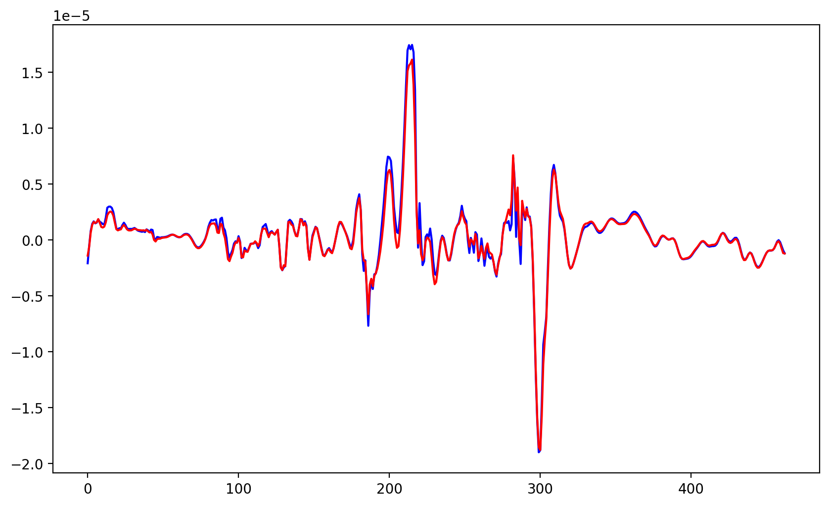
• 可以发现两种方法的曲线基本一致

方法检验

对于两种计算方法的计算结果进行检验，前面也简单画了一下图，下面主要从空间分布图以及任意选择一个空间点的时间序列来检验其计算结果是否存在差异。

空间分布图

def plot_contour(ax, data, label, lon, lat, levels, cmap='RdYlGn', transform=ccrs.PlateCarree(), extend='both'):
   
    cs = ax.contourf(lon, lat, data, levels=levels, cmap=cmap, transform=transform, extend=extend)
    ax.coastlines()
    ax.add_feature(cfeature.BORDERS)
    ax.set_title(label)
    box = [100,120,10,20]
    ax.set_extent(box,crs=ccrs.PlateCarree())
    ax.set_xticks(np.arange(box[0],box[1], 10), crs=transform)
    ax.set_yticks(np.arange(box[2], box[3], 5), crs=transform)
    ax.xaxis.set_major_formatter(LongitudeFormatter())
    ax.yaxis.set_major_formatter(LatitudeFormatter())
    plt.colorbar(cs, ax=ax, orientation='horizontal')
    ax.set_aspect(1)
# 创建画布和子图
fig, (ax1, ax2, ax3) = plt.subplots(1, 3, figsize=(16, 6),dpi=200, subplot_kw={'projection': ccrs.PlateCarree()})

# 绘制三个不同的图
plot_contour(ax1, tadv[0] * 10**4, 'Metpy', lon, lat, levels=np.linspace(-1, 1, 21))
plot_contour(ax2, padv[0] * 10**4, 'Numpy', lon, lat, levels=np.linspace(-1, 1, 21))
plot_contour(ax3, (np.array(tadv[0]) - padv[0]) * 10**4, 'difference',
             lon, lat, 
             levels=11)

# 显示图形
plt.tight_layout()
plt.show()

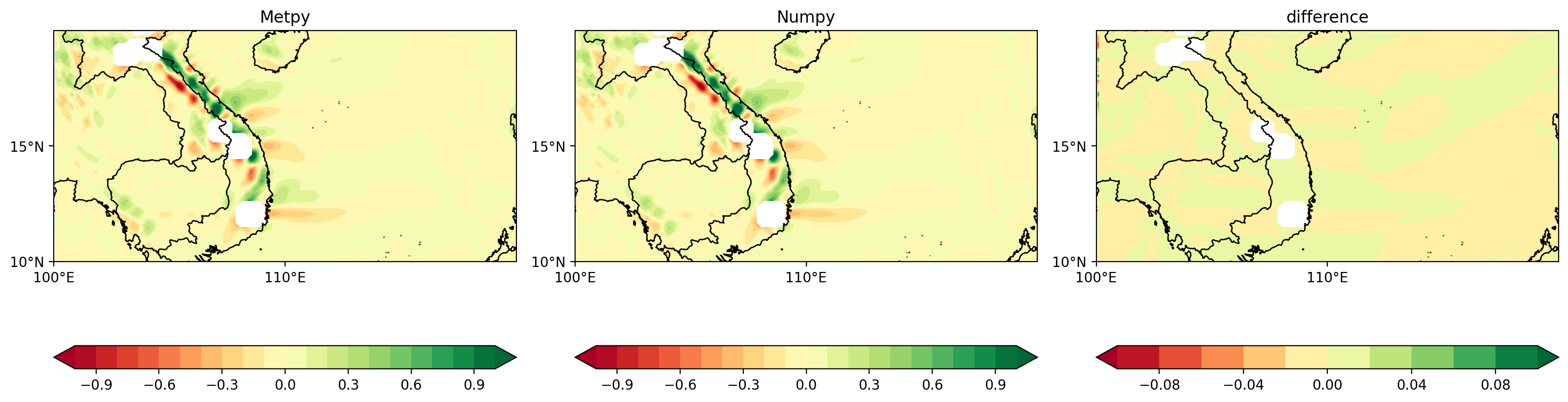
• 子图1为metpy计算结果，子图2为numpy计算结果，子图3为两种计算结果的差异
• 为了保证结果可靠性，前两个子图选择相同的量级，绘制间隔(levels)，colormap

可以发现，整体上对于第一个时刻的pv平流项空间分布图，两种方法的计算结果整体上是一致的，说明两种计算方法都是可行的；两种计算方法的差异小于0.01，在一定程度上可以忽略，不影响整体结论以及后续的分析。

任意空间点的时间序列

def extract_time_series(lon, lat, lon0, lat0, tadv, padv2):
    def find_nearest(array, value):
        array = np.asarray(array)
        idx = (np.abs(array - value)).argmin()
        return idx

    lon_idx = find_nearest(lon, lon0)
    lat_idx = find_nearest(lat, lat0)
    
    tadv_series = tadv[:, lat_idx, lon_idx] * 10**4
    padv2_series = padv2[:, lat_idx, lon_idx] * 10**4
    diff_series = (np.array(tadv[:, lat_idx, lon_idx]) - padv2[:, lat_idx, lon_idx]) * 10**4
    
    return tadv_series, padv2_series, diff_series

lon0, lat0 = 100, 15  # 根据实际需要修改

# 提取该点的时间序列数据
tadv_series, padv_series, diff_series = extract_time_series(lon, lat, lon0, lat0, tadv, padv)

# 创建新的画布绘制时间序列曲线
plt.figure(figsize=(10, 6),dpi=200)
plt.plot(tadv_series, label='Metpy')
plt.plot(padv_series, label='Numpy')
plt.plot(diff_series, label='Diff')
plt.xlabel('Time')
plt.ylabel('Value')
plt.legend()
plt.title(f'Time Series at Point ({lon0}, {lat0})')
plt.grid(True)
plt.show()

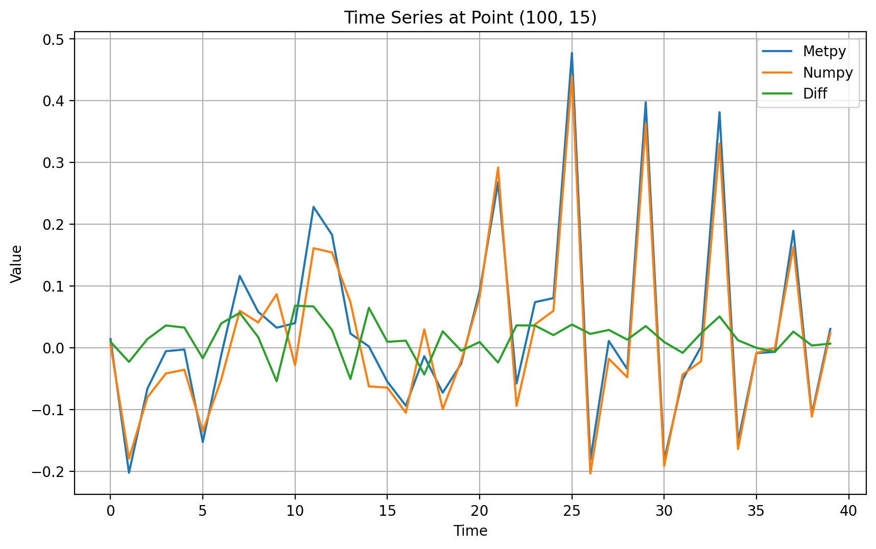
• 从任意空间点的时间序列检验上，可以发现两种计算方法差异基本一致，总体上Metpy的结果稍微高于numpy的计算方法，可以和地球半径以及pi的选择有关
• 从差异上来看，总体上在-0.1~0.1之间，误差可以忽略，不会影响主要的结论

总结

• 这里，通过基于Metpy和Numpy的方法分别计算了位涡的平流项，并绘制了空间分布图以及任意空间点时间序列曲线来证明两种方法的有效性，在计算过程我们需要重点关注的是单位是否为国际基本度量单位，这里避免我们的计算的结果的量级的不确定性；
• 当然，这里仅仅是收支方程中的一项，我们可以在完整的计算整个收支方程的各项结果后，比较等号两端的单位是否一致，来证明收支方程结果的有效性。

单位查阅：https://unidata.github.io/MetPy/latest/tutorials/unit_tutorial.html
advection：https://unidata.github.io/MetPy/latest/api/generated/metpy.calc.advection.html