使用python+gdal实现arcgis的核密度分析，针对点密度

最新推荐文章于 2024-05-20 18:36:09 发布

gis_rc

最新推荐文章于 2024-05-20 18:36:09 发布

阅读量3.4k

点赞数 5

分类专栏： gdal 文章标签： python

本文链接：https://blog.csdn.net/weixin_44265800/article/details/111572804

版权

gdal 专栏收录该内容

4 篇文章 1 订阅

订阅专栏

核密度分析的工作原理：核密度分析工具用于计算要素在其周围邻域中的密度。此工具既可计算点要素的密度，也可计算线要素的密度
可能的用途包括针对社区规划分析房屋密度或犯罪行为，或探索道路或公共设施管线如何影响野生动物栖息地。可使用 population
字段赋予某些要素比其他要素更大的权重，该字段还允许使用一个点表示多个观察对象。例如，一个地址可以表示一栋六单元的公寓，或者在确定总体犯罪率时可赋予某些罪行比其他罪行更大的权重。对于线要素，分车道高速公路可能比狭窄的土路具有更大的影响。
核密度分析用于计算每个输出栅格像元周围的点要素的密度。
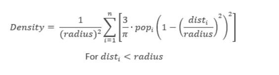
概念上，每个点上方均覆盖着一个平滑曲面。在点所在位置处表面值最高，随着与点的距离的增大表面值逐渐减小，在与点的距离等于搜索半径的位置处表面值为零。仅允许使用圆形邻域。曲面与下方的平面所围成的空间的体积等于此点的 Population 字段值，如果将此字段值指定为 NONE 则体积为每个输出栅格像元的密度均为叠加在栅格像元中心的所有核表面的值之和。核函数以 Silverman 的著作（1986 年版，第 76 页，equation 4.5）中描述的四次核函数为基础。
如果 population 字段设置使用的是除 NONE 之外的值，则每项的值用于确定点被计数的次数。例如，值 3
会导致点被算作三个点。值可以为整型也可以为浮点型。
默认情况下，单位是根据输入点要素数据的投影定义的线性单位进行选择的，或是在输出坐标系环境设置中以其他方式指定的。
公式：

核密度公式
详细的信息请到arcgis灌完的在线帮助查看

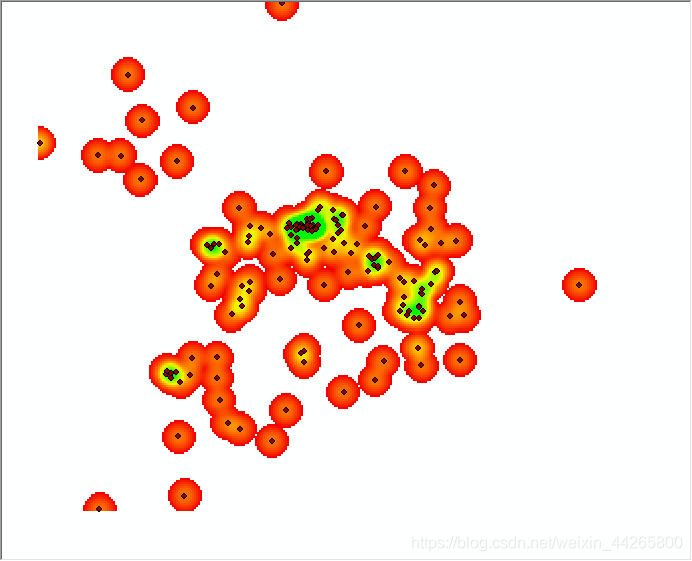
我这里提供了两种实现的方式，最主要的不同就是点的半径的判断
1.图像长宽小的一边除以30

def KernelDensity(ref_raster, points_shp_file, region_shp, calc_field, out_raster, radius=None, pixel_size=None):
    """
    :param ref_raster: 参考栅格
    :param points_shp_file: 点shp文件
    :param calc_field: 核密度计算字段，表示遍布于用来创建连续表面的景观内的计数或数量。
    :param radius: 搜索半径，默认值为输出空间参考中输出范围的宽度或高度的最小值除以 30。
    :param pixel_size: 输出的像元大小，默认为参考栅格的像元大小
    :return: 核密度结果栅格文件
    """
    # 1.点转栅格
    ratio_result_file = m_cfg["ratio_result"] + r"/工业GDP系数.tif"
    if os.path.exists(ratio_result_file):
        return ratio_result_file
    raster_from_points = pointsToRaster(points_shp_file, ref_raster, calc_field, pixel_size)
    dataset = gdal.Open(raster_from_points, gdalconst.GA_ReadOnly)
    dataset_geo_trans = dataset.GetGeoTransform()
    x_min = dataset_geo_trans[0]
    y_max = dataset_geo_trans[3]
    x_res = dataset_geo_trans[1]
    col = dataset.RasterXSize
    row = dataset.RasterYSize

    min_col_row = col if col < row else row
    radius = (min_col_row / 30) * x_res if radius == None else radius
    # 2.开始计算
    raster_data = dataset.GetRasterBand(1).ReadAsArray()
    points_xy = []
    values = []
    point_shp_ds = ogr.GetDriverByName("ESRI Shapefile").Open(points_shp_file, 0)
    if point_shp_ds is None:
        print("文件{0}打开失败！".format(points_shp_file))
        return
    points_layer = point_shp_ds.GetLayer(0)
    feature_count = points_layer.GetFeatureCount()
    for i in range(feature_count):
        feature = points_layer.GetFeature(i)
        feature_defn = points_layer.GetLayerDefn()
        calc_field_index = feature_defn.GetFieldIndex(calc_field)
        field_value = feature.GetField(calc_field_index)
        values.append(field_value)
        point_xy = feature.GetGeometryRef()
        points_xy.append([point_xy.GetX(), point_xy.GetY()])

    radius_pixel_width = int(radius / abs(x_res))
    out_ds = dataset.GetDriver().Create(out_raster, col, row, 1,
                                        dataset.GetRasterBand(1).DataType)  # 创建一个构建重采样影像的句柄
    out_ds.SetProjection(dataset.GetProjection())  # 设置投影信息
    out_ds.SetGeoTransform(dataset_geo_trans)  # 设置地理变换信息
    result_data = np.full((row, col), -999.000, np.float32)  # 设置一个与重采样影像行列号相等的矩阵去接受读取所得的像元值
    ratio_data = np.full((row, col), -999.0, np.float32)
    region_shp_ds = ogr.GetDriverByName("ESRI Shapefile").Open(region_shp, 0)
    region_layer = region_shp_ds.GetLayer(0)
    region_feature_count = region_layer.GetFeatureCount()

    all_k_points=[]
    for i in range(len(points_xy)):

        x_pos = int((points_xy[i][0] - x_min) / abs(x_res))
        y_pos = int((y_max - points_xy[i][1]) / abs(x_res))
        # 先搜索以点为中心正方形区域，再在里面搜索圆形
        y_len_min = (y_pos - radius_pixel_width - 1) if (y_pos - radius_pixel_width - 1) > 0 else 0
        y_len_max = (y_pos + radius_pixel_width + 1) if (y_pos + radius_pixel_width + 1) < row else row

        x_len_min = (x_pos - radius_pixel_width - 1) if (x_pos - radius_pixel_width - 1) > 0 else 0
        x_len_max = (x_pos + radius_pixel_width + 1) if (x_pos + radius_pixel_width + 1) < col else col
        for y in range(y_len_min, y_len_max):
            for x in range(x_len_min, x_len_max):
                distance = ((x - x_pos) ** 2 + (y - y_pos) ** 2) ** 0.5
 				# 判断在半径内
                if (distance < radius):
                    value = raster_data[y_pos][x_pos]
                    scale = (distance * x_res) / radius
                    D_value = (3 * (1 - scale ** 2) ** 2) / (math.pi * (radius ** 2)) * value
                    if (result_data[y][x] != -999.0):
                        result_data[y][x] += D_value
                    else:
                        result_data[y][x] = D_value

    out_band = out_ds.GetRasterBand(1)
    out_band.WriteArray(result_data)
    out_band.SetNoDataValue(-999)
    out_band.FlushCache()
    out_band.ComputeStatistics(False)  # 计算统计信息
    out_ds.BuildOverviews('average', [1, 2, 4, 8, 16, 32])  # 构建金字塔

    result_data[result_data<0]=0
    result_data=result_data/sum(values)
    result_data[result_data==0]=-999
    array2raster(out_ds, result_data, ratio_result_file, col, row)
    return ratio_result_file

核密度分析

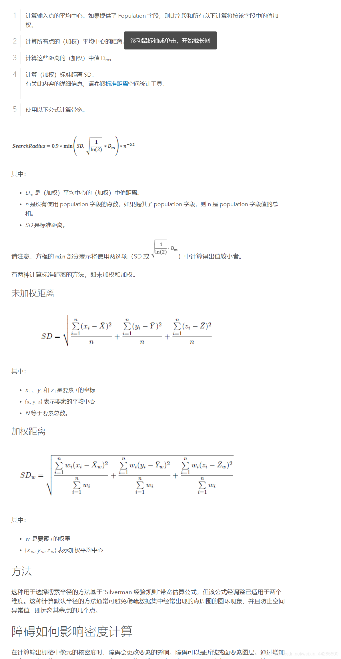
2.使用“Silverman 经验规则”的空间变量专为输入数据集计算默认搜索半径（带宽），该变量可有效避免空间异常值（即距离其余点太远的点）。详细的讲解可以看arcgis的在线帮助
在这里插入图片描述

def KernelDensity(ref_raster, points_shp_file, calc_field, out_raster, radius=None, pixel_size=None):
    """
    :param ref_raster: 参考栅格
    :param points_shp_file: 点shp文件
    :param calc_field: 核密度计算字段，表示遍布于用来创建连续表面的景观内的计数或数量。
    :param radius: 搜索半径，默认值为输出空间参考中输出范围的宽度或高度的最小值除以 30。
    :param pixel_size: 输出的像元大小，默认为参考栅格的像元大小
    :return: 核密度结果栅格文件
    """
    # try:
    # 1.点转栅格
    raster_from_points = pointsToRaster(points_shp_file, ref_raster, calc_field, pixel_size)
    dataset = gdal.Open(raster_from_points, gdalconst.GA_ReadOnly)
    dataset_geo_trans = dataset.GetGeoTransform()
    x_min = dataset_geo_trans[0]
    y_max = dataset_geo_trans[3]
    x_res = dataset_geo_trans[1]
    print(dataset_geo_trans)
    col = dataset.RasterXSize
    row = dataset.RasterYSize

    min_col_row = col if col < row else row
    # 2.开始计算
    raster_data = dataset.GetRasterBand(1).ReadAsArray()
    points_xy = []
    point_shp_ds = ogr.GetDriverByName("ESRI Shapefile").Open(points_shp_file, 0)
    if point_shp_ds is None:
        print("文件{0}打开失败！".format(points_shp_file))
        return
    points_layer = point_shp_ds.GetLayer(0)
    feature_count = points_layer.GetFeatureCount()
    pointXs = []
    pointYs = []
    values=[]
    for i in range(feature_count):
        feature = points_layer.GetFeature(i)
        feature_defn = points_layer.GetLayerDefn()
        calc_field_index = feature_defn.GetFieldIndex(calc_field)
        field_value = feature.GetField(calc_field_index)
        values.append(field_value)
        point_xy = feature.GetGeometryRef()
        points_xy.append([point_xy.GetX(), point_xy.GetY()])
        pointXs.append(point_xy.GetX()*field_value)
        pointYs.append(point_xy.GetY()*field_value)
    # 1.计算输入点的平均中心。如果提供了 Population 字段，则此字段和所有以下计算将按该字段中的值加权。
    mean_x = sum(pointXs) / len(pointXs)
    mean_y = sum(pointYs) / len(pointYs)
    # 2.计算所有点的（加权）平均中心的距离。
    weight_distances = []
    standerd_x = 0
    standerd_y=0
    for i in range(len(points_xy)):
        standerd_x+=(abs(points_xy[i][0]*values[i] - mean_x)) ** 2
        standerd_y+=abs(points_xy[i][1]*values[i] - mean_y)**2
        w_distance = (abs((points_xy[i][0]*values[i]) ** 2 - mean_x ** 2) + abs((points_xy[i][1]*values[i]) ** 2 - mean_y ** 2)) ** 0.5
        weight_distances.append(w_distance)
    # 3.计算这些距离的（加权）中值 Dm。
    p_median = np.median(weight_distances)
    SDm=math.sqrt(1/np.log(2))*p_median
    # 4.计算（加权）标准距离 SD。
    SD=(standerd_x/len(points_xy)+standerd_y/len(points_xy)/len(points_xy))**0.5
	
    search_radius=0.9*min(SD,SDm)*((1/len(points_xy))**0.2)
    radius = search_radius if radius == None else radius
    out_ds = dataset.GetDriver().Create(out_raster, col, row, 1,
                                        dataset.GetRasterBand(1).DataType)  # 创建一个构建重采样影像的句柄
    out_ds.SetProjection(dataset.GetProjection())  # 设置投影信息
    out_ds.SetGeoTransform(dataset_geo_trans)  # 设置地理变换信息
    result_data = np.full((row, col), -999.000, np.float32)  # 设置一个与重采样影像行列号相等的矩阵去接受读取所得的像元值

    for i in range(len(points_xy)):
    	#动态的搜索半径，这里是加权后的搜索半径，
        radius_pixel_width=int(search_radius/values[i])
        x_pos = int((points_xy[i][0] - x_min) / abs(x_res))
        y_pos = int((y_max - points_xy[i][1]) / abs(x_res))
        # 先搜索以点为中心正方形区域，再在里面搜索圆形
        y_len_min = (y_pos - radius_pixel_width - 1) if (y_pos - radius_pixel_width - 1) > 0 else 0
        y_len_max = (y_pos + radius_pixel_width + 1) if (y_pos + radius_pixel_width + 1) < row else row

        x_len_min = (x_pos - radius_pixel_width - 1) if (x_pos - radius_pixel_width - 1) > 0 else 0
        x_len_max = (x_pos + radius_pixel_width + 1) if (x_pos + radius_pixel_width + 1) < col else col

        for y in range(y_len_min, y_len_max):
            for x in range(x_len_min, x_len_max):
                distance = ((x - x_pos) ** 2 + (y - y_pos) ** 2) ** 0.5*values[i]
                # 判断在半径内
                if (distance < radius):
                    value = raster_data[y_pos][x_pos]
                    scale = (distance * x_res) / radius
                    D_value = (3 * (1 - scale ** 2) ** 2) / (math.pi * (radius ** 2)) * value
                    if (result_data[y][x] != -999.0):
                        result_data[y][x] += D_value
                    else:
                        result_data[y][x] = D_value


    out_band = out_ds.GetRasterBand(1)
    out_band.WriteArray(result_data)
    out_band.SetNoDataValue(-999)
    out_band.FlushCache()
    out_band.ComputeStatistics(False)  # 计算统计信息
    out_ds.BuildOverviews('average', [1, 2, 4, 8, 16, 32])  # 构建金字塔
    del dataset  # 删除句柄
    del out_ds
    return out_raster

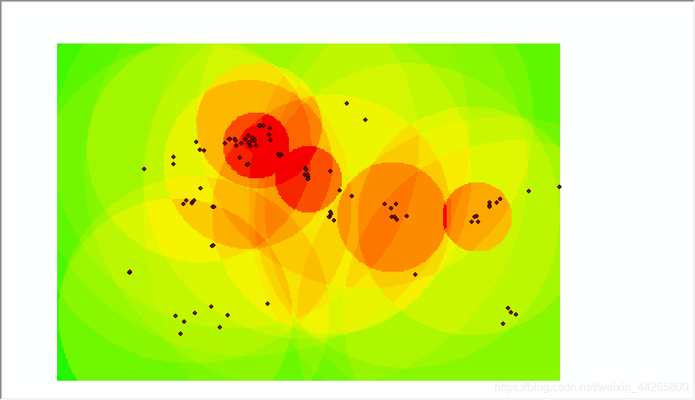
我这里值太大了，搜索半径就会特别的广，这也是正常的，如果你一个点代表了很多的人，肯定分布的区域也会增大很多
在这里插入图片描述

# 点转栅格
def pointsToRaster(points_shp_file, in_raster, filed_value, pixel_size=None):
    """
    :param points_shp_file: 点shp文件
    :param in_raster: 输入参照栅格，一定得是坐标系统为4326的栅格文件
    :param filed_value: 赋值字段
    :param pixel_size: 输出的像元大小
    :return: 结果栅格文件
    """
    try:
        result_tif = 'result_' + str(uuid.uuid4()) + '.tif'
        if pixel_size != None:
            in_raster = resampleRaster(in_raster, pixel_size)
        dataset = gdal.Open(in_raster, gdalconst.GA_ReadOnly)

        geo_transform = dataset.GetGeoTransform()
        cols = dataset.RasterXSize  # 列数
        rows = dataset.RasterYSize  # 行数

        shp = ogr.Open(points_shp_file, 0)
        m_layer = shp.GetLayerByIndex(0)
        out_file = m_cfg["temp_path"] + r"/toraster_{0}.tif".format(str(uuid.uuid4()))
        target_ds = gdal.GetDriverByName('GTiff').Create(out_file, xsize=cols, ysize=rows, bands=1,
                                                         eType=gdal.GDT_Float32)
        target_ds.SetGeoTransform(geo_transform)
        target_ds.SetProjection(dataset.GetProjection())

        band = target_ds.GetRasterBand(1)
        band.SetNoDataValue(-999)
        band.FlushCache()
        gdal.RasterizeLayer(target_ds, [1], m_layer, options=["ATTRIBUTE=" + filed_value])  # 跟shp字段给栅格像元赋值
        del dataset
        shp.Release()
        print('转栅格完成！')
        return out_file
    except Exception as e:
        print("转栅格出错:{0}".format(str(e)))
        return

# 重新设置栅格像元大小
def resampleRaster(in_raster, pixel_size):
    """
    :param in_raster: 输入栅格
    :param pixel_size: 输出的像元大小
    :return: 结果栅格文件
    """
    try:
        in_ds = gdal.Open(in_raster)
        out_raster = m_cfg["temp_path"] + r"/resample_{0}.tif".format(str(uuid.uuid4()))
        geotrans = list(in_ds.GetGeoTransform())
        ratio = geotrans[1] / pixel_size
        geotrans[1] = pixel_size  # 像元宽度变为原来的两倍
        geotrans[5] = -pixel_size  # 像元高度也变为原来的两倍
        in_band = in_ds.GetRasterBand(1)
        xsize = in_band.XSize
        ysize = in_band.YSize
        x_resolution = int(xsize * ratio)+1  # 影像的行列都变为原来的一半
        y_resolution = int(ysize * ratio)+1
        out_ds = in_ds.GetDriver().Create(out_raster, x_resolution, y_resolution, 1,
                                          in_band.DataType)  # 创建一个构建重采样影像的句柄
        out_ds.SetProjection(in_ds.GetProjection())  # 设置投影信息
        out_ds.SetGeoTransform(geotrans)  # 设置地理变换信息
        data = np.empty((y_resolution, x_resolution), np.float32)  # 设置一个与重采样影像行列号相等的矩阵去接受读取所得的像元值
        in_band.ReadAsArray(buf_obj=data)
        out_band = out_ds.GetRasterBand(1)
        out_band.WriteArray(data)
        out_band.SetNoDataValue(-999)
        out_band.FlushCache()
        out_band.ComputeStatistics(False)  # 计算统计信息
        out_ds.BuildOverviews('average', [1, 2, 4, 8, 16, 32])  # 构建金字塔
        del in_ds  # 删除句柄
        del out_ds
        print("重设栅格大小成功")
        return out_raster
    except Exception as e:
        print("重设栅格大小出错{0}".format(str(e)))
        return

# 根据计算后的数组生成tif
def array2raster(dataset, data, out_file, x_size, y_size):
    if os.path.exists(out_file):
        return out_file
    out_ds = dataset.GetDriver().Create(out_file, x_size, y_size, 1,
                                        dataset.GetRasterBand(1).DataType)  # 创建一个构建重采样影像的句柄
    out_ds.SetProjection(dataset.GetProjection())  # 设置投影信息
    out_ds.SetGeoTransform(dataset.GetGeoTransform())  # 设置地理变换信息
    out_band = out_ds.GetRasterBand(1)
    out_band.WriteArray(data)
    out_band.SetNoDataValue(-999)
    out_band.FlushCache()
    out_band.ComputeStatistics(False)  # 计算统计信息
    out_ds.BuildOverviews('average', [1, 2, 4, 8, 16, 32])  # 构建金字塔
    del dataset  # 删除句柄
    del out_ds
    return out_file

gis_rc

关注

5
点赞
踩
29

收藏

觉得还不错? 一键收藏
13
评论
使用python+gdal实现arcgis的核密度分析，针对点密度

核密度分析的工作原理：核密度分析工具用于计算要素在其周围邻域中的密度。此工具既可计算点要素的密度，也可计算线要素的密度可能的用途包括针对社区规划分析房屋密度或犯罪行为，或探索道路或公共设施管线如何影响野生动物栖息地。可使用 population 字段赋予某些要素比其他要素更大的权重，该字段还允许使用一个点表示多个观察对象。例如，一个地址可以表示一栋六单元的公寓，或者在确定总体犯罪率时可赋予某些罪行比其他罪行更大的权重。对于线要素，分车道高速公路可能比狭窄的土路具有更大的影响。核密度分析用于计算每个输出栅
复制链接

扫一扫