分布函数相关

$f(\cdot )$ is a PDF with support $(0,a)$. $a$ being possibly $+\infty$， CDF is $F(\cdot )$

关于期望的有用表达式

$$E[X]={\int }_0^{a}xf(x)dx={\int }_0^{a}xdF(x)={\int }_0^a(1-F(x))dx$$
前两个等号很容易得出，下面证明：
proof：
$$\begin{array}{rl}{\int }_0^{a}xdF(x)& =-{\int }_0^{a}xd(1-F(x))\\ & =-x(1-F(x)){|}_0^a+{\int }_0^a(1-F(x))dx\\ & ={\int }_0^a(1-F(x))dx\end{array}$$
第二个等式的第一个式子为0。实际上用的是分布积分的内容。$\square$
另外根据相似的证明，可以得到
$${\int }_0^{b}xf(x)dx=bF(b)-{\int }_0^{b}F(x)dx,\forall b<a$$

联合分布函数的导数和偏导数

假设两个连续随机变量 $X,Y$, 联合分布函数定义为
$$F_{X,Y}(x,y)=P(X\le x,Y\le y)={\int }_{-\infty }^x{\int }_{-\infty }^y{f}_{X,Y}(t_1,t_2)d{t}_{1}d{t}_2$$
众所周知
$$\frac{{\partial }^2{F}_{X,Y}(x,y)}{\partial x\partial y}=f_{X,Y}(x,y)$$
偏导数
$$\begin{array}{rl}\frac{\partial F_{X,Y}(x,y)}{\partial x}& ={\int }_{-\infty }^y{f}_{X,Y}(x,t)dt\\ & ={\int }_{-\infty }^y{f}_{Y|X=x}(t)f_X(x)dt\\ & ={\int }_{-\infty }^y{f}_{Y|X=x}(t)dt{f}_X(x)\\ & =F_{Y|X=x}(y)f_X(x)\\ & =F_Y(y)f_{X|Y\le y}(x)\end{array}$$
最后一行是因为
$${\int }_{-\infty }^y{f}_{X,Y}(x,t)dt={\int }_{-\infty }^y{f}_Y(t)f_{X|Y=t}(x)dt$$

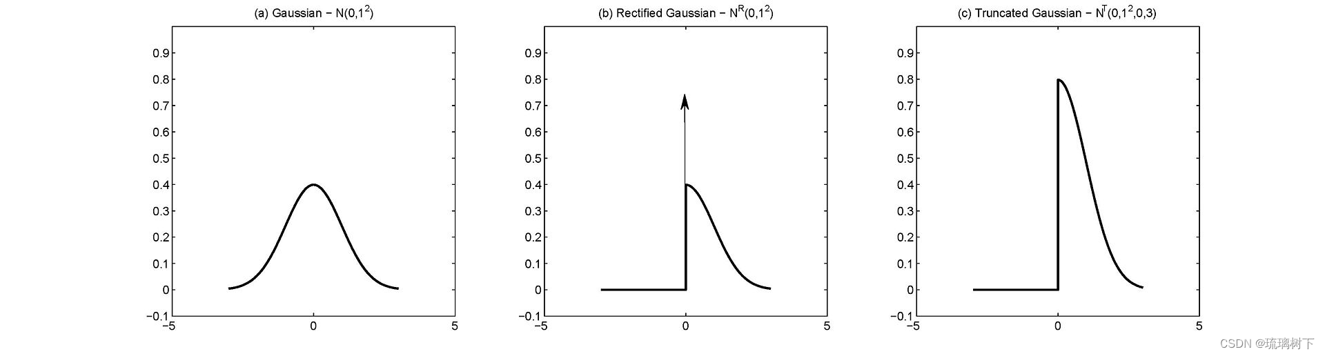
高斯分布相关

高斯分布 (Gaussian/Normal Distribution)

PDF：
$$f(x;\mu ,\sigma )=\frac{1}{\sigma \sqrt{2\pi }}{e}^{-\frac{1}{2}(\frac{x-\mu }{\sigma }{)}^2}$$
CDF:
$$F(x)=\Phi (\frac{x-\mu }{\sigma })$$

Rectified Gaussian Distribution

PDF:
$$h(x)=\{\begin{array}{rl}f(x),& x>0\\ 0,& x\le 0\end{array}$$
CDF:
$$H(x)=\Phi (\frac{x-\mu }{\sigma })-\Phi (-\frac{\mu }{\sigma })$$

Truncated Gaussian Distribution

如果设定的范围是 [a,b]
PDF:
$$g(x;\mu ,\sigma ,a,b)=\{\begin{array}{rl}\frac{f(x)}{\Phi (\frac{b-\mu }{\sigma })-\Phi (\frac{a-\mu }{\sigma })},& x\in [a,b]\\ 0,& otherwise\end{array}$$
三者的区别：
图源：Bayesian non-negative factor analysis for reconstructing transcription factor mediated regulatory networks

Folded Gaussian distribution

PDF:
$$l(x;\mu ,\sigma )=\{\begin{array}{rl}\frac{1}{\sigma \sqrt{2\pi }}{e}^{-\frac{1}{2}(\frac{x-\mu }{\sigma }{)}^2}+\frac{1}{\sigma \sqrt{2\pi }}{e}^{-\frac{1}{2}(\frac{x+\mu }{\sigma }{)}^2},& x\ge 0\\ 0,& otherwise\end{array}$$