Python实现一元线性回归——不调包

一元线性回归

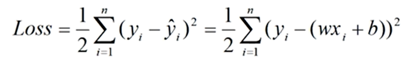
损失函数/代价函数（Loss/cost function）：模型的预测值与真实值的不一致程度
平方损失函数（square loss）

要使得Loss最小，根据极值点的偏导为零，联立方程组。
对未知的两个变量求偏导然后联立方程组

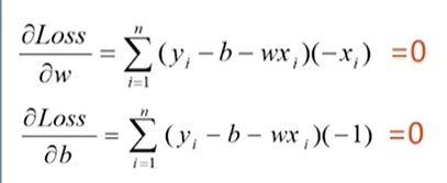
求解得到两种不同形式的结果，但实际上是等价的结果。

利用Python实现计算一元线性回归（所有的点的坐标已知，求拟合函数的权重和偏置值）

x = [137.97,104.50,100.00,124.32,79.2,99.,124.,114.,106.69,138.05,53.75,46.91,68.,63.02,81.26,86.21]
y = [145.,110.,93.,116.,65.32,104.,118.,91.,62.,133.,51.,45.,78.5,69.65,75.69,95.3]

# 计算平均值
meanX = sum(x)/len(x)
meanY = sum(y)/len(y)

# 计算权重的分子和分母
sumXY = 0.0
sumX = 0.0
for i in range(len(x)):
    sumXY += (x[i]-meanX)*(y[i]-meanY)
    sumX += (x[i]-meanX) *(x[i]-meanX)

w = sumXY/sumX # 计算权重
b = meanY-w*meanX # 计算偏置值

print('w=',w,' b=',b)

用numpy数组实现

import numpy as np

x = [137.97,104.50,100.00,124.32,79.2,99.,124.,114.,106.69,138.05,53.75,46.91,68.,63.02,81.26,86.21]
y = [145.,110.,93.,116.,65.32,104.,118.,91.,62.,133.,51.,45.,78.5,69.65,75.69,95.3]
x = np.array(x)
y = np.array(y)

meanX = np.mean(x)
meanY = np.mean(y)

# 计算权重的分子和分母
sumXY = np.sum((x-meanX)*(y-meanY))
sumX = np.sum((x-meanX)*(x-meanX))



w = sumXY/sumX # 计算权重
b = meanY-w*meanX # 计算偏置值
print('w=',w,' b=',b)

用TensorFlow实现

import tensorflow as tf

x = [137.97,104.50,100.00,124.32,79.2,99.,124.,114.,106.69,138.05,53.75,46.91,68.,63.02,81.26,86.21]
y = [145.,110.,93.,116.,65.32,104.,118.,91.,62.,133.,51.,45.,78.5,69.65,75.69,95.3]
x = tf.constant(x)
y = tf.constant(y)

meanX = tf.reduce_mean(x)
meanY = tf.reduce_mean(y)

# 计算权重的分子和分母
sumXY = tf.reduce_sum((x-meanX)*(y-meanY))
sumX = tf.reduce_sum((x-meanX)*(x-meanX))


w = sumXY/sumX # 计算权重
b = meanY-w*meanX # 计算偏置值
print('w=',w.numpy(),' b=',b.numpy())

完整实现

import tensorflow as tf
import numpy as np
import matplotlib.pyplot as plt

#设置图像中显示中文
plt.rcParams['font.sans-serif'] = ['SimHei']

x = [137.97,104.50,100.00,124.32,79.2,99.,124.,114.,106.69,138.05,53.75,46.91,68.,63.02,81.26,86.21]
y = [145.,110.,93.,116.,65.32,104.,118.,91.,62.,133.,51.,45.,78.5,69.65,75.69,95.3]
x = tf.constant(x)
y = tf.constant(y)

meanX = tf.reduce_mean(x)
meanY = tf.reduce_mean(y)

# 计算权重的分子和分母
sumXY = tf.reduce_sum((x-meanX)*(y-meanY))
sumX = tf.reduce_sum((x-meanX)*(x-meanX))


w = sumXY/sumX # 计算权重
b = meanY-w*meanX # 计算偏置值
print('权值w=',w.numpy(),'\n偏置值b=',b.numpy())
print('线性模型：y=',w.numpy(),'*x+',b.numpy())

x_test = np.array([128.15,45.,141.43,106.27,99.,53.84,85.36,70.])
y_pred = (w*x_test+b).numpy()
print('面积\t估计房价')
n=len(x_test)
for i in range(n):
    print(x_test[i],'\t',round(y_pred[i],2)) # round()四舍五入

#可视化
plt.figure() # 创建画布

plt.scatter(x,y,color="red",label="销售记录")
plt.scatter(x_test,y_pred,color="blue",label="预测房价")
plt.plot(x_test,y_pred,color="green",label="拟合直线",linewidth=2)

plt.xlabel("面积(平方米)")
plt.ylabel("价格(万元)")

#坐标轴范围
plt.xlim((40,150))
plt.ylim((40,150))

plt.suptitle("商品房销售价格评估预测",fontsize=20)

plt.legend(loc="upper left") # 左上方显示图例
plt.show()

结果