java图数据结构

概念：

图G＝（V，E）由一组顶点V和一组边E组成，每一条边是一个元组（v，w），其中v,w属于V中。如果对元组有序的，则图是有向的(directed)。否则图是无向的(undirected)。

在无向图中(undirected graph)，边是没有方向的平面线。在无向图中，可以沿着边任意走一条路。任何无向图都可以表示为有向图，方法是用两条有向边替换每一条无向边。

在有向图中(directed graph)，有向图是指每一条边上的顶点都是有序的图。边是从一个节点指向另一个节点的箭头。<Vi,Vj>：Vi称为尾部，Vj称为头部。在有向图中, 只能按照箭头的方向从一个节点转到另一个节点。这意味着, 在有向图中, 有可能达到死胡同, 也有可能到达一个你不能离开的节点。

完全图(complete graph)是每对顶点之间都有一条边的图。无向完全图：n个顶点和n（n-1）/2条边。有向完全图：n个顶点和n（n-1）边。如果（u，v）是E（G）中的边，则u与v相邻，v与v相邻。

加权图(weoghted graph)：有时边有第三个组成部分, 重量或成本, 其语义是特定于图形的。具有与其边缘关联的值的图称为加权图。该图可以是定向的, 也可以是无方向的。权重可以表示如下内容:两个顶点之间的物理距离。从一个顶点到另一个顶点所需的时间。从顶点到顶点的行程成本是多少。

子图(Subgraph)：子图设G=（V，E）是顶点集V和边集E的图。G的子图是图G'=（V'，E'），其中

1. V'是V的一个子集。
2. E'由E中的边（v，w）组成，使得v和w都在V'中(子图中的边要预先存在，并且定点在子图中)

顶点的度(degree)：顶点v的度是连接到顶点v的边数，记为TD(v)。在有向图中，顶点度是进度和出度之和：顶点v的入度是头部为顶点v的边的数目，记为ID(v);顶点v的出度是尾部为顶点v的边数，记为OD(v)

路径的长度是在未加权的图形中沿着路径的边数。它是加权图中路径上弧线的成本之和。

环是在同一顶点处开始和结束的边 (v, v).且其长度大于等于1 。

简单路径是路径上的各顶点均不互相重复。

DAG(定向无环图):无环有向图(图不包含环，若图不包含环，则为无环图)

连通图：连通图是一个无向图，其中有一条从每个顶点到其余另一个顶点的路径。

1. 强连通图是一个有向图，其中每个顶点之间都有一条路径(考虑方向)
2. 弱连通图是一个有向图，它不是强连通的，但如果图被转换成无向图，它就会连通（简单地忽略方向）。

图的连通分量( Connected Component)：无向图G的极大连通子图称为G的连通分量。任何连通图的连通分量只有一个，即是其自身，非连通的无向图有多个连通分量。

1. 有向图的一个强连通分量是一个极大的顶点集(不一定包含所有的顶点，可以是多个)，其中有一条从集合中任何一个顶点到集合中任何其他顶点的路径。
2. 在非连通的无向图中, 从其中的顶点开始只能访问同一连通分量中的顶点 (最大的连通子图)搜索所有连接的组件搜索图形中的每个顶点。如果已访问该顶点, 则它必须位于连通分量中。否则, 从这个顶点开始遍历图形, 我们将得到另一个连通分量。

生成树：如果连通图G的一个子图是一棵包含G的所有顶点的树，则该子图称为G的生成树。 每个具有 n 个顶点的生成树都包含完全为 n-1 的边。如果我们在树上添加任何边缘, 我们就会得到一个循环。

对于无向图G和一棵树T来说，如果T是G的子图，则称T为G的树，如果T是G的生成子图，则称T是G的生成树。

最小生成树：对于一个边上具有权值的图来说，其边权值和最小的生成树称做图G的最小生成树(包含所有节点)。对于一个图G，如果图中的边权值都不相同，则图的最小生成树唯一。

有向树：在根树T中，出度为零的点称为树叶

1. 有且仅有一个结点的入度为0；
2. 除树根外的结点入度为1；
3. 从树根到任一结点有一条有向通路，T中其他顶点称为内点或支点。在根树中，有时需要考虑同一层上结点的次序，规定了每一层上的结点的次序的根树称为有序树。

实现：

 

数据结构的定义：

由于图中存储了图的顶点和路径信息，所以其数据结构也应该保存相应的信息。

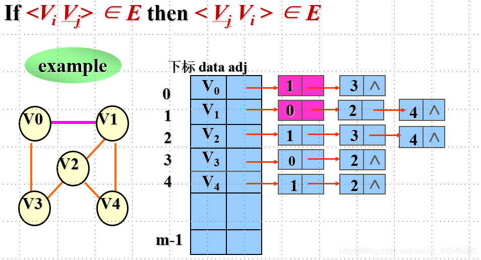
故使用邻接矩阵存储信息，其顶点映射到整数0..N-1，而边则映射成一个N*N的矩阵，定义如下：

对于有向图与无向图而言：

对于加权图而言：

 

代码实现

 第一种方式：矩阵实现

缺点：空间复杂度高，O(N^2),实际生活中们并不适用

import java.util.LinkedList;
import java.util.Queue;
import java.util.Stack;

//浪费空间，有O(N^2)的空间复杂度
public class GraphMatrix<Type> {
	private static int MAXV=10;
	private Vetex<Type>[] vetex;
	private int[][] edges;
	private int currentv;
	public GraphMatrix() {
		this.vetex=new Vetex[MAXV];
		this.edges=new int[MAXV][MAXV];
		currentv=0;
		for(int i=0;i<MAXV;i++) {
			for(int j=0;j<MAXV;j++) {
				this.edges[i][j]=0;
			}
		}
	}
	public boolean isEmpty() {
		return currentv==0;
	}
	public boolean isFull() {
		return this.currentv==MAXV-1;
	}
	public int sizev() {
		return currentv+1;
	}
	public int sizee() {
		int sum=0;
		for(int i=0;i<=this.currentv;i++) {
			for( int j=0;j<=this.currentv;j++) {
				sum+=edges[i][j];
			}
		}
		return sum;
	}
	public void addv(Type data) {
		if(find(data)!=-1) {
			System.out.println("顶点"+data+"已添加");
		}else {
			this.vetex[this.currentv]=new Vetex<>(data);
			this.currentv++;
		}	
	}
	public void adde(Type start,Type end) {
		int start1=find(start);
		int end1=find(end);
		if(start1!=-1 && end1!=-1) {
			this.edges[start1][end1]=1;
			this.edges[end1][start1]=1;
		}else {
			System.out.println(start+"或"+end+"不存在");
		}
	}
	public int find(Type data) {
		System.out.println("长度为："+this.currentv);
		for(int i=0;i<this.currentv;i++) {
			if(data.equals(vetex[i].data)) {
				return i;
			}
		}
		return -1;
	}
	public void print() {
		for( int i=0;i<this.currentv;i++) {
			for( int j=0;j<this.currentv;j++) {
				System.out.print(this.edges[i][j]+" ");
			}
			System.out.println();
		}
	}
	//广度优先遍历
	public void bfs() {
		Queue<Integer> q=new LinkedList<>();
		q.add(0);
		this.vetex[0].isVisited=true;
		System.out.print(this.vetex[0].data+" ");
		while(!q.isEmpty()) {
			int res=q.poll();
			int x;
			while(( x=findFirst(res))!=-1) {
				System.out.print(this.vetex[x].data+" ");
				this.vetex[x].isVisited=true;
				q.add(x);
			}
			
		}
		System.out.println();
		for(int i=0;i<this.currentv;i++) {
			this.vetex[i].isVisited=false;
		}
	}
	//深度优先便利
	public void dfs() {
		Stack<Integer> s=new Stack<>();
		System.out.print(this.vetex[0].data+" ");
		s.push(0);
		vetex[0].isVisited=true;
		while(!s.isEmpty()) {
			int res=findFirst(s.peek());
			if(res==-1) {
				s.pop();
			}else {
				System.out.print(this.vetex[res].data+" ");
				s.push(res);
				this.vetex[res].isVisited=true;
			}
			
		}
		System.out.println();
		for(int i=0;i<this.currentv;i++) {
			this.vetex[i].isVisited=false;
		}
	}
	public int findFirst(int index) {
		for(int i=0;i<this.currentv;i++) {
			if(this.edges[index][i]==1 && (!this.vetex[i].isVisited)) {
				return i;
			}
		}
		return -1;
	}
	
}
class Vetex<Type>{
	public Type data;
	public boolean isVisited;
	public Vetex() {
		this.data=null;
		this.isVisited=false;
	}
	public Vetex(Type data) {
		this.data=data;
		this.isVisited=false;
	}
}

class TestGraphMatrix{
	public static void main(String args[]) {
		GraphMatrix<Character> graph = new GraphMatrix<>();
        graph.addv('A');
        graph.addv('B');
        graph.addv('C');
        graph.addv('D');
        graph.addv('E');
        graph.adde('B', 'C');
        graph.adde('A', 'B');
        graph.adde('C', 'D');
        graph.adde('B', 'E');
        graph.adde('C', 'E');
        graph.print();
        graph.dfs();
         graph.bfs();

	}
}

第二种实现(基于链表的实现)

概念：

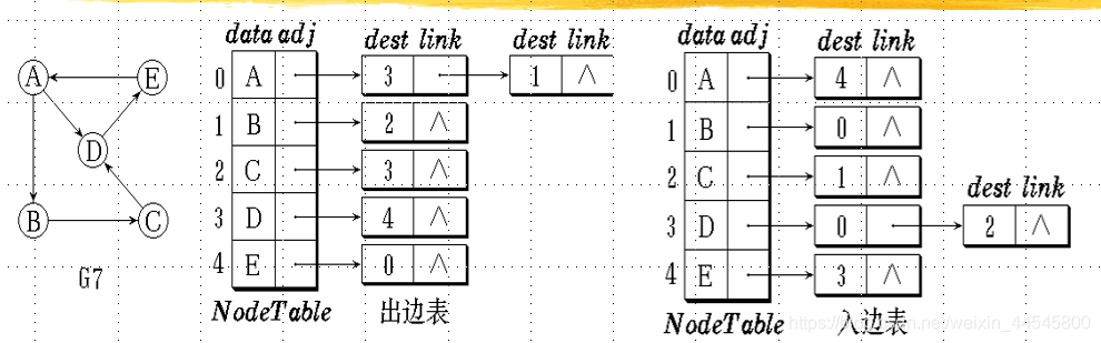
无向图邻接矩阵：

1. 无向图的邻接矩阵是对称的。在邻接列表表示形式中, 如果 (i, j) 是边, 则顶点 j 在顶点 i 列表中, 顶点 i 在顶点 j 列表中。

有向图邻接矩阵：

1. 在邻接列表中，第i个边列表表示从顶点i开始的所有边。
2. 在逆邻接列表中，第i个列表中的所有边都以顶点i结束。

代码实现：
 

 

两种实现方式比较：

如果图形是稀疏的, 并且边缘不多, 则邻接列表可能比邻接矩阵更具有空间效率。

如果图形是密集的, 并且边缘的数量是 O(N2), 那么邻接矩阵可能会更有效的空间。

空间复杂度：

矩阵形式：O(V^2)

import java.util.LinkedList;
import java.util.Queue;

import ds.sequence.SeqList;

public class GraphLink<Type> {
	private static int SIZE=10; 
	private SeqList<VetexNode<Type>> graph;
	private int currente;
	public GraphLink() {
		this.graph=new SeqList<>(SIZE);
		this.currente=0;
	}
	public boolean isEmpty() {
		return this.graph.size()==0;
	}
	public void makeEmpty() {
		this.graph.makeEmpty();
	}
	 
	public int sizev() {
		return this.graph.size();
	}
	public int sizee() {
		return this.currente;
	}
	public void addv(Type data) {
		graph.add(this.graph.size(), new VetexNode<>(data));
	}
	public void adde(Type datav,Type datae) {
		int resv=find(datav);
		int rese=find(datae);
		if(resv==-1) {
			addv(datav);
		}
		if(rese==-1) {
			addv(datae);
		}
		if(resv!=-1 && rese!=-1) {
			EdgeNode v=graph.get(find(datav)).nodev;
			if(v==null) {
				graph.get(find(datav)).nodev=new EdgeNode(rese);
			}else {
				while(v.nodee!=null) {
					v=v.nodee;
				}
				v.nodee=new EdgeNode(rese);
			}
			
			EdgeNode v2=graph.get(find(datae)).nodev;
			if(v2==null) {
				graph.get(find(datae)).nodev=new EdgeNode(resv);
			}else {
				while(v2.nodee!=null) {
					v2=v2.nodee;
				}
				v2.nodee=new EdgeNode(resv);
			}
			this.currente++;
		}
	}
	public void bfs() {  //广度遍历
		boolean [] visited = new boolean[graph.size()];   //需要另开辟一个数组，若每一个顶点都保存一个isvisited的话，由于每个节点地址不同，依旧会重复输出。
		for(int i=0;i<visited.length;i++) {
			visited[i]=false;
		}
		Queue<Integer> q=new LinkedList<>();
		q.add(0);
		System.out.print(graph.get(0).data+" ");
		visited[0]=true;
		while(!q.isEmpty()) {
			int res=q.poll();
			EdgeNode v=this.graph.get(res).nodev;
			while(v!=null) {
				if(!visited[v.dest]) {
					q.add(v.dest);
					visited[v.dest]=true;
					System.out.print(graph.get(v.dest).data+" ");
				}
				v=v.nodee;
			}
			
		}
		System.out.println();
		
	}
	
	//输出连通分量   
	public void components() {
		//类似于深度遍历，只不过得把所有的额顶点全部遍历完成
		System.out.println("略");
	}
	
	public int find(Type data) {
		for( int i=0;i<this.graph.size();i++) {
			if(data.equals(this.graph.get(i).data)) {
				return i;
			}
		}
		return -1;
	}
}
class EdgeNode{
	public int dest;
	public int weight;
	public EdgeNode nodee;
	public EdgeNode() {
		this.nodee=null;
	}
	public EdgeNode(int dest) {
		this.dest=dest;
	}
	public EdgeNode(int dest,int weight) {
		this.dest=dest;
		this.weight=weight;
		this.nodee=null;
	}
	public EdgeNode(int dest, int weight, EdgeNode node) {
		this.dest = dest;
		this.weight = weight;
		this.nodee = node;
	}
	
}
class VetexNode<Type>{
	public Type data;
	public EdgeNode nodev;
	public VetexNode() {
		this.data=null;
		this.nodev=null;
	}
	public VetexNode(Type data) {
		this.data=data;
		this.nodev=null;
	}
	public VetexNode(Type data, EdgeNode nodev) {
		this.data = data;
		this.nodev = nodev;
	}
	
}
class TestGraphLink{
	public static void main(String args[]) {
		GraphLink<Character> graph=new GraphLink<>();
		graph.addv('A');
        graph.addv('B');
        graph.addv('C');
        graph.addv('D');
        graph.addv('E');
        graph.adde('B', 'C');
        graph.adde('A', 'B');
        graph.adde('C', 'D');
        graph.adde('B', 'E');
        graph.adde('C', 'E');
        graph.adde('A', 'C');
        System.out.println("共有"+graph.sizee()+"条路径");
         graph.bfs();
	}
}

邻接表形式：O(V+N)

时间复杂度：

 

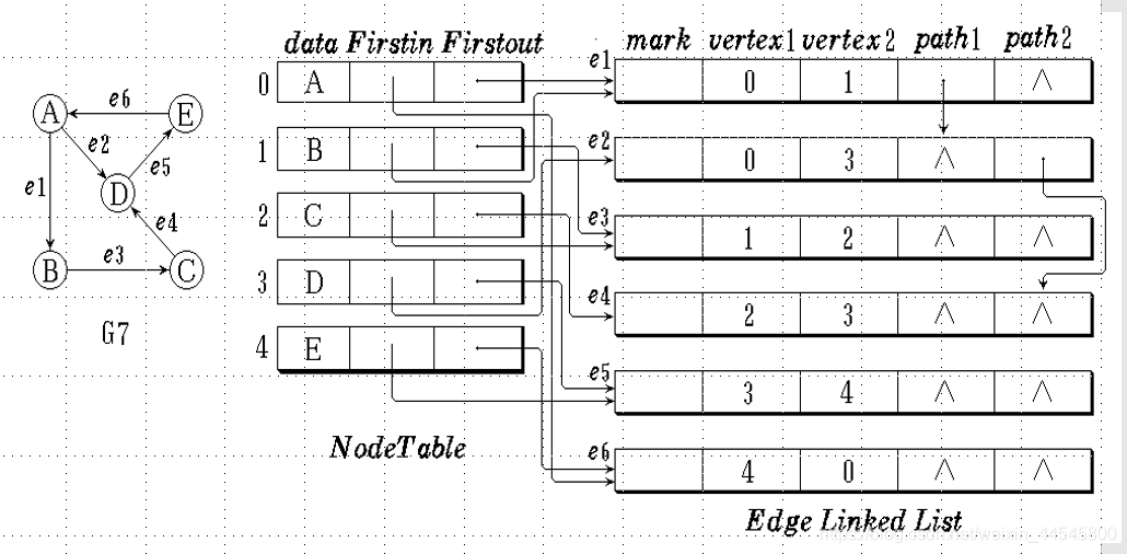
临界多表

无向图的邻接多表

在无向图的邻接多重表中，每一条边被一个边节点表示。所以遍历图就变得很遍历，而顶点列表是顺序列表。每个节点有两个成员。数据存储有关顶点的信息，从该顶点到第一条边的第一个输出点

结构如下：

eg:

 

有向图的临界多表：

path1：指向与此顶点具有相同源的下一个顶点。
path2：指向与此顶点具有相同目标的下一个顶点。

由节点表示的每个顶点。它是边内列表和边外列表的头
member：存储有关此顶点的信息。
Firstin：指向此顶点的第一个边端点
Firstout：指出此顶点的第一个边端点

eg: