


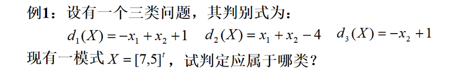
一、线性分类–判断该函数属于哪一类
先上例题,然后我会通过两种方法来判断该函数属于哪一类
1、图解法
定义
对于多类问题:模式有 ω1 ,ω2 , … , ωm 个类别,可分三种情况:
第一种情况:每一模式类与其它模式类间可用单个判别平面把一个类分开。这种情况,M类可有M个判别函数,且具有以下性质:
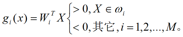

下图所示,每一类别可用单个判别边界与其它类别相分开 。如果一模式X属于ω1,则由图可清楚看出:这时g1(x) >0而g2(x) <0 , g3(x) <0 。ω1 类与其它类之间的边界由 g1(x)=0确定。
 详解
详解

2、python代码
def determine(x1,x2):#x1,x2表示模式x=[7,5]^t
    d1x=d1[0]*x1+d1[1]*x2+d1[1]
    d2x=d2[0]*x1+d2[1]*x2+d2[1]
    d3x=d3[0]*x1+d1[1]*x2+d3[1]
    if d1x>0:
        print("该判定结果:X∈ω1")
    elif d2x>0:
        print("该判定结果:X∈ω2")
    elif d3x>0:
        print("该判定结果:X∈ω3")
    else:
        print("分类失败")
d1=[-1,1,1]#表示d1的系数和截距
d2=[1,1,-4]#表示d2的系数和截距
d3=[-1,1,0]#表示d3的系数和截距
determine(7,5)

二、Fisher线性分类
1、Fisher的概念和几何意义
Fisher判别法是判别分析的方法之一,它是借助于方差分析的思想,利用已知各总体抽取的样品的p维观察值构造一个或多个线性判别函数y=l′x其中l= (l1,l2…lp)′,x= (x1,x2,…,xp)′,使不同总体之间的离差(记为B)尽可能地大,而同一总体内的离差(记为E)尽可能地小来确定判别系数l=(l1,l2…lp)′。数学上证明判别系数l恰好是|B-λE|=0的特征根,记为λ1≥λ2≥…≥λr>0。所对应的特征向量记为l1,l2,…lr,则可写出多个相应的线性判别函数,在有些问题中,仅用一个λ1对应的特征向量l1所构成线性判别函数y1=l′1x不能很好区分各个总体时,可取λ2对应的特征向量l′2建立第二个线性判别函数y2=l′2x,如还不够,依此类推。有了判别函数,再人为规定一个分类原则(有加权法和不加权法等)就可对新样品x判别所属

python代码
import pandas as pd
import numpy as np
import matplotlib.pyplot as plt
import seaborn as sns
path=r'media/Iris.csv'
df = pd.read_csv(path, header=0)
Iris1=df.values[0:50,0:4]
Iris2=df.values[50:100,0:4]
Iris3=df.values[100:150,0:4]
m1=np.mean(Iris1,axis=0)
m2=np.mean(Iris2,axis=0)
m3=np.mean(Iris3,axis=0)
s1=np.zeros((4,4))
s2=np.zeros((4,4))
s3=np.zeros((4,4))
for i in range(0,30,1):
    a=Iris1[i,:]-m1
    a=np.array([a])
    b=a.T
    s1=s1+np.dot(b,a)
for i in range(0,30,1):
    c=Iris2[i,:]-m2
    c=np.array([c])
    d=c.T
    s2=s2+np.dot(d,c)
    #s2=s2+np.dot((Iris2[i,:]-m2).T,(Iris2[i,:]-m2))
for i in range(0,30,1):
    a=Iris3[i,:]-m3
    a=np.array([a])
    b=a.T
    s3=s3+np.dot(b,a)
sw12=s1+s2
sw13=s1+s3
sw23=s2+s3
#投影方向
a=np.array([m1-m2])
sw12=np.array(sw12,dtype='float')
sw13=np.array(sw13,dtype='float')
sw23=np.array(sw23,dtype='float')
#判别函数以及T
#需要先将m1-m2转化成矩阵才能进行求其转置矩阵
a=m1-m2
a=np.array([a])
a=a.T
b=m1-m3
b=np.array([b])
b=b.T
c=m2-m3
c=np.array([c])
c=c.T
w12=(np.dot(np.linalg.inv(sw12),a)).T
w13=(np.dot(np.linalg.inv(sw13),b)).T
w23=(np.dot(np.linalg.inv(sw23),c)).T
#print(m1+m2) #1x4维度  invsw12 4x4维度  m1-m2 4x1维度
T12=-0.5*(np.dot(np.dot((m1+m2),np.linalg.inv(sw12)),a))
T13=-0.5*(np.dot(np.dot((m1+m3),np.linalg.inv(sw13)),b))
T23=-0.5*(np.dot(np.dot((m2+m3),np.linalg.inv(sw23)),c))
kind1=0
kind2=0
kind3=0
newiris1=[]
newiris2=[]
newiris3=[]
for i in range(30,49):
    x=Iris1[i,:]
    x=np.array([x])
    g12=np.dot(w12,x.T)+T12
    g13=np.dot(w13,x.T)+T13
    g23=np.dot(w23,x.T)+T23
    if g12>0 and g13>0:
        newiris1.extend(x)
        kind1=kind1+1
    elif g12<0 and g23>0:
        newiris2.extend(x)
    elif g13<0 and g23<0 :
        newiris3.extend(x)
#print(newiris1)
for i in range(30,49):
    x=Iris2[i,:]
    x=np.array([x])
    g12=np.dot(w12,x.T)+T12
    g13=np.dot(w13,x.T)+T13
    g23=np.dot(w23,x.T)+T23
    if g12>0 and g13>0:
        newiris1.extend(x)
    elif g12<0 and g23>0:

        newiris2.extend(x)
        kind2=kind2+1
    elif g13<0 and g23<0 :
        newiris3.extend(x)
for i in range(30,50):
    x=Iris3[i,:]
    x=np.array([x])
    g12=np.dot(w12,x.T)+T12
    g13=np.dot(w13,x.T)+T13
    g23=np.dot(w23,x.T)+T23
    if g12>0 and g13>0:
        newiris1.extend(x)
    elif g12<0 and g23>0:
        newiris2.extend(x)
    elif g13<0 and g23<0 :
        newiris3.extend(x)
        kind3=kind3+1
correct=(kind1+kind2+kind3)/60
print("样本类内离散度矩阵S1:",s1,'\n')
print("样本类内离散度矩阵S2:",s2,'\n')
print("样本类内离散度矩阵S3:",s3,'\n')
print('-----------------------------------------------------------------------------------------------')
print("总体类内离散度矩阵Sw12:",sw12,'\n')
print("总体类内离散度矩阵Sw13:",sw13,'\n')
print("总体类内离散度矩阵Sw23:",sw23,'\n')
print('-----------------------------------------------------------------------------------------------')
print('判断出来的综合正确率:',correct*100,'%')
结果显示:


2、鸢尾花数据集的分类
数据集准备
首先先从网上下载鸢尾花数据集,读者可以通过下列网址直接下载:
添加链接描述
python代码
首先导入要用到的库
import numpy as np
from sklearn.linear_model import LogisticRegression
import matplotlib.pyplot as plt
import matplotlib as mpl
from sklearn import preprocessing
import pandas as pd
from sklearn.preprocessing import StandardScaler
from sklearn.pipeline import Pipeline
对各个变量进行赋值,取出数据集(注意这里我是将数据集放到D盘下的,请更改自己数据集具体地址或复制粘贴到D盘下)
import numpy as np
from sklearn.linear_model import LogisticRegression
import matplotlib.pyplot as plt
import matplotlib as mpl
from sklearn import preprocessing
import pandas as pd
from sklearn.preprocessing import StandardScaler
from sklearn.pipeline import Pipeline

df = pd.read_csv("D:\iris.data", header=0)
x = df.values[:, :-1]
y = df.values[:, -1]
print('x = \n', x)
print('y = \n', y)
le = preprocessing.LabelEncoder()
le.fit(['Iris-setosa', 'Iris-versicolor', 'Iris-virginica'])
print(le.classes_)
y = le.transform(y)
print('Last Version, y = \n', y)
构建线性模型
x = x[:, :2]
x = StandardScaler().fit_transform(x)
lr = LogisticRegression()   # Logistic回归模型
lr.fit(x, y.ravel())        # 根据数据[x,y],计算回归参数
鸢尾花数据集的分类可视化
N, M = 500, 500     # 横纵各采样多少个值
x1_min, x1_max = x[:, 0].min(), x[:, 0].max()   # 第0列的范围
x2_min, x2_max = x[:, 1].min(), x[:, 1].max()   # 第1列的范围
t1 = np.linspace(x1_min, x1_max, N)
t2 = np.linspace(x2_min, x2_max, M)
x1, x2 = np.meshgrid(t1, t2)                    # 生成网格采样点
x_test = np.stack((x1.flat, x2.flat), axis=1)   # 测试点
cm_light = mpl.colors.ListedColormap(['#77E0A0', '#FF8080', '#A0A0FF'])
cm_dark = mpl.colors.ListedColormap(['g', 'r', 'b'])
y_hat = lr.predict(x_test)       # 预测值
y_hat = y_hat.reshape(x1.shape)                 # 使之与输入的形状相同
plt.pcolormesh(x1, x2, y_hat, cmap=cm_light)     # 预测值的显示
plt.scatter(x[:, 0], x[:, 1], c=y.ravel(), edgecolors='k', s=50, cmap=cm_dark)
plt.xlabel('petal length')
plt.ylabel('petal width')
plt.xlim(x1_min, x1_max)
plt.ylim(x2_min, x2_max)
plt.grid()
plt.savefig('2.png')
plt.show()
计算该线性分类器模型的准确率
y_hat = lr.predict(x)
y = y.reshape(-1)
result = y_hat == y
acc = np.mean(result)
print('准确度: %.2f%%' % (100 * acc))
结果显示


 276
276


 被折叠的 条评论
为什么被折叠?
被折叠的 条评论
为什么被折叠?
 到【灌水乐园】发言


