


However, first we’ll start this chapter by talking about storage engines that are used in the kinds of databases that you’re probably familiar with: traditional relational databases, and also most so-called NoSQL databases. We will examine two families of storage engines: log-structured storage engines, and page-oriented storage engines such as B-trees.
Data Structures That Power Your Database
The simplest database in the world is two Bash functions:
#!/bin/bash
db_set () {
  echo "$1,$2" >> database
}

db_get () {
  grep "^$1," database | sed -e "s/^$1,//" | tail -n 1
}
Every call to db_set appends to the end of a file, when you update a key, the old version is not overwritten–you need to look at the last occurrence of a key in a file to find the latest value. db_set has pretty good performance, because appending to a file is generally very efficient. Many databases internally use a log, just like db_set does. But it still has some shortages:
- its performance will be terrible if you have a large number of records in your database. Every time you want to look up a key,
db_gethas to scan the entire database file from beginning to end. - more issues to deal with (such as concurrency control, reclaiming disk space so that the log doesn’t grow forever, and handling errors and partially written records),
In order to efficiently find the value for a particular key in the database, we need a different data structure: an index.
Hash Indexes
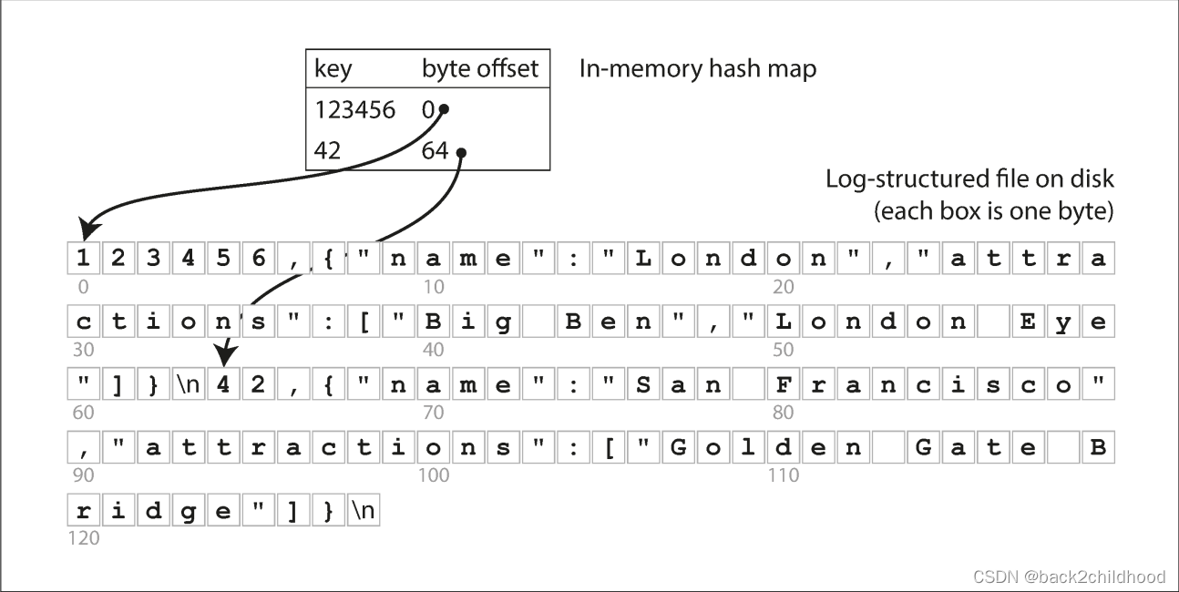
The simplest possible indexing strategy is: keeping an in-memory hash map where every key is mapped to a byte offset in the data file----the location at which the value can be found. Whenever you append a new key-value pair to the file, you also update the hash map to reflect the offset of the data you just wrote(this works both for inserting new keys and for updating existing keys). When you want to look up a value, use the hash map to find the offset in the data file, seek to that location, and read the value.
If you want to delete a key and its associated value, you have to append a special deletion record to the data file (sometimes called a tombstone).
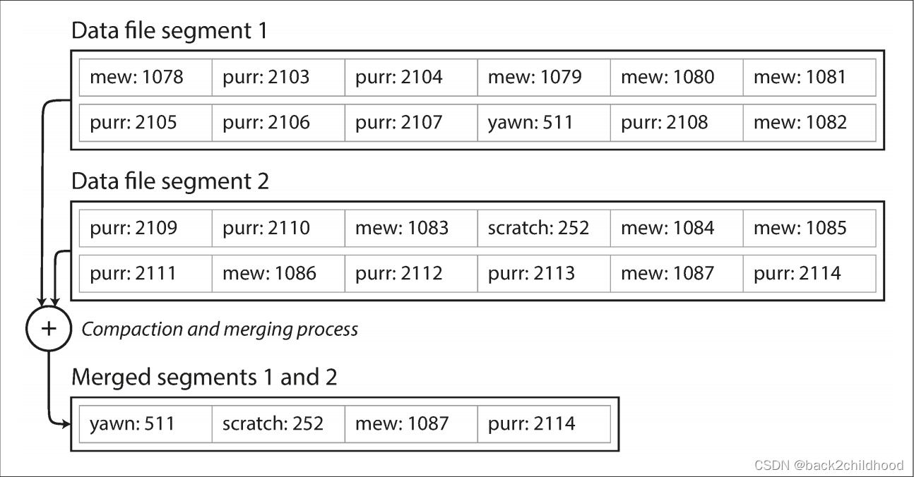
We can break the log into segments of a certain size by closing segment file when it reaches a certain size to avoid eventally running out of disk space. Moreover, since compaction often makes segments much smaller (assuming that a key is overwritten several times on average within one segment), we can also merge several segments together at the same time as performing the compaction.
In order to achieve concurrency control, there is only one writer thread. Data file segments are append-only and otherwise immutable, so they can be read concurrently by multiple threads.
- Good
- Appending and segment merging are sequential write operations, which are generally much faster than random writes, especially on magnetic spinning-disk hard drives. To some extent, sequential writes are also preferable on flash-based
solid state drives(SSDs). - Merging old segments avoids the problem of data files getting fragmented over time.
- Concurrency and crash recovery are much simpler if segment files are append-only or immutable. For example, you don’t have to worry about the case where a crash happened while a value was being overwritten, leaving you with a file containing part of the old and part of the new value spliced together.
- Appending and segment merging are sequential write operations, which are generally much faster than random writes, especially on magnetic spinning-disk hard drives. To some extent, sequential writes are also preferable on flash-based
- Limitations
- Range queries are not efficient. you’d have to look up each key individually in the hash maps.
- The hash table must fit in memory, so the number of keys shouldn’t be too large or small.
SSTables and LSM-Trees
- Sorted String Table(SSTable): the sequence of key-value pairs is sorted by key.
- advantages:
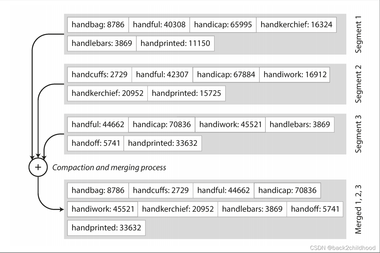
- Merging segments is simple and efficient, even if the files are bigger than the available memory. This approach is like
mergesortalgorithm.
- In order to find a particular value, you no longer need to keep an index of all the keys in memory. If you are looking for the key
b, but don’t know the exact offset of that key in the segment file. However, you do know the offsets of the keysaandc, so you can jump to the offset foraand scan from there until you findb.
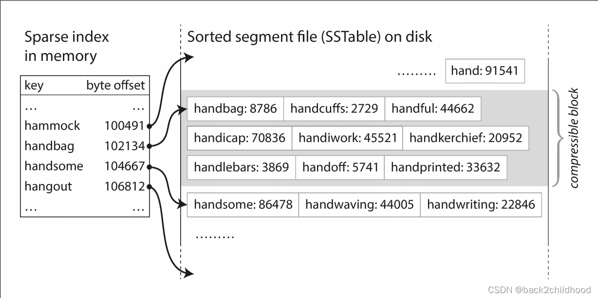
- Since read requests need to scan over several key-value pairs in the requested range anyway, it is possible to group those records into a block and compress it before writing it to disk.
- Merging segments is simple and efficient, even if the files are bigger than the available memory. This approach is like
Constructing and maintaining SSTables
- When a write comes in, add it to an in-memory balanced tree data structure (for example, a red-black tree). This in-memory tree is called a
memtable. - When the memtable is bigger than a threshold----typically a few megabytes----write it out to disk as an SSTable file. This can be done efficiently because the tree maintains sorted by key.
- In order to serve a read request, first try to find the key in the memtable, then in the most recent on-disk segment, then in the older segment.
- From time to time, run a merging and compaction process in the background to combine segment files and discard overwritten and deleted values.
- We can keep a separate log on disk to which every write is immediately appended, that log is not in sorted order, because its only purpose is to restore the memtable after a crash.
Making an LSM-tree out of SSTables
Performance optimizations
- If you want to look for a key do not exist in the database: you have to check the memtable, then the segments all the way back to the oldest(possibly having to read from disk for each one) before you can be sure that the key does not exist. In order to optimize, we can use
Bloom filters. - There are also different strategies to determine the order and timing of how SSTables are compacted and merged:
- size-tiered compaction: newer and smaller SSTables are successively merged into older and larger SSTables.
- leveled compaction: the key range is split up into smaller SSTables and older data is moved into separate “levels,” which allows the compaction to proceed more incrementally and use less disk space.
B-Trees
Like SSTables, B-trees keep key-value pairs sorted by key, which allows efficient key-value lookups and range queries. B-trees break the database down into fixed-size blocks or pages, traditionally 4KB in size, and read or write one page at a time.
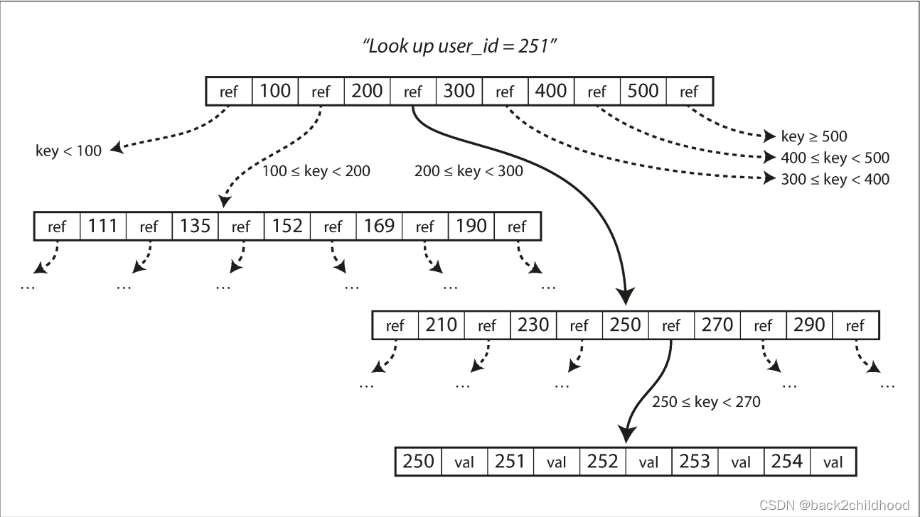
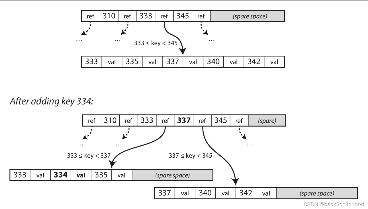
If you want to add a new key, you need to find the page whose range encompasses the new key and add it to that page. If there isn’t enough space in the page to accommodate the new key, it is split into two half-full pages, and the parent page is updated to account for the new subdivision of key ranges.
This algorithm ensures the tree remains balanced: a B-tree with n keys always has a depth of O(log n). Most databases can fit into a B-tree that is three or four levels deep, so you don’t need to follow many page references to find the page you are looking for. (A four-level tree of 4 KB pages with a branching factor of 500 can store up to 256 TB.)
Making B-trees reliable
If you split a page because you want to insert a new key, this is a dangerous operation, because if the database crashes after only some of the pages be written, you end up with a corrupted index.
In order to make the database more reliable, there are two implementations:
- write-ahead log(WAL, also know as redo log). This is an append-only file to which every B-tree modification must be written before it can be written to the tree itself. When the database comes back up after a crash, this log is used to restore the B-tree back to a consistent state.
- Concurrency control is required if multiple threads are going to access the B-tree at the same time,
latches(lightweight locks)is used to protect the tree’s data structures.
B-tree optimizations
- Instead of overwriting pages and maintaining a WAL for crash recovery, some databases (like LMDB) use a copy-on-write scheme.
- We can save space in pages by not storing the entire key, but abbreviating it.
- Additional pointers have been added to the tree. For example, each leaf page may have references to its sibling pages to the left and right, which allows scanning keys in order without jumping back to parent pages.
Comparing B-Trees and LSM-Trees
Advantages of LSM-trees
- A B-tree index must write every piece of data at least twice: once to the write-ahead log, and once to the tree page itself (and perhaps again as pages are split).
- Log-structured indexes also rewrite data multiple times due to repeated compaction and merging of SSTables. This effect—one write to the database resulting in multiple writes to the disk over the course of the database’s lifetime—is known as write amplification. Moreover, LSM-trees are typically able to sustain higher write throughput than B-trees, partly because they sometimes have lower write amplification.
- LSM-trees can be compressed better, and thus often produce smaller files on disk than B-trees. B-tree storage engines leave some disk space unused due to fragmentation.
Downsides of LSM-trees
- A downside of log-structured storage is that the compaction process can sometimes interfere with the performance of ongoing reads and writes.
- Another issue with compaction arises at high write throughput: the disk’s finite write bandwidth needs to be shared between the initial write (logging and flushing a memtable to disk) and the compaction threads running in the background. If write throughput is high and compaction is not configured carefully, in this case, the number of unmerged segments on disk keeps growing until you run out of disk space, and reads also slow down because they need to check more segment files.
- An advantage of B-trees is that each key exists in exactly one place in the index, whereas a log-structured storage engine may have multiple copies of the same key in different segments.
Other Indexing Structures
So far we have only discussed key-value indexes, which are like a primary key index in the relational model.
It is also common to have secondary index, you can use CREATE INDEX to create a secondary index.
A secondary index can easily be constructed from a key-value index. The main difference is that keys are not unique.
Storing values within the index
Multi-column indexes
Keeping everything in memory
As RAM becomes cheaper, the cost-per-gigabyte argument is eroded. Many datasets are simply not that big, so it’s quite feasible to keep them entirely in memory.
Besides performance, in-memory databases also provide data models that are difficult to implement with disk-based indexes. For example, Redis offers a database-like interface to various data structures such as priority queues and sets. Because it keeps all data in memory, its implementation is comparatively simple.
Transaction Processing or Analytics?

There was a trend for companies to stop using their OLTP systems for analytics purposes, and to run the analytics on a separate database instead. This separate database was called a data warehouse.
Data Warehousing
A data warehouse, by contrast, is a separate database that analysts can query to their hearts’ content, without affecting OLTP operations. The data warehouse contains a read-only copy of the data in all the various OLTP systems in the company. Data is extracted from OLTP databases (using either a periodic data dump or a continuous stream of updates), transformed into an analysis-friendly schema, cleaned up, and then loaded into the data warehouse. This process of getting data into the warehouse is known as Extract–Transform–Load (ETL).

The divergence between OLTP databases and data warehouses
Stars and Snowflakes: Schemas for Analytics
- Star schema: The name “star schema” comes from the fact that when the table relationships are visualized, the fact table is in the middle, surrounded by its dimension tables.
- A variation of this template is known as the snowflake schema, where dimensions are further broken down into subdimensions.
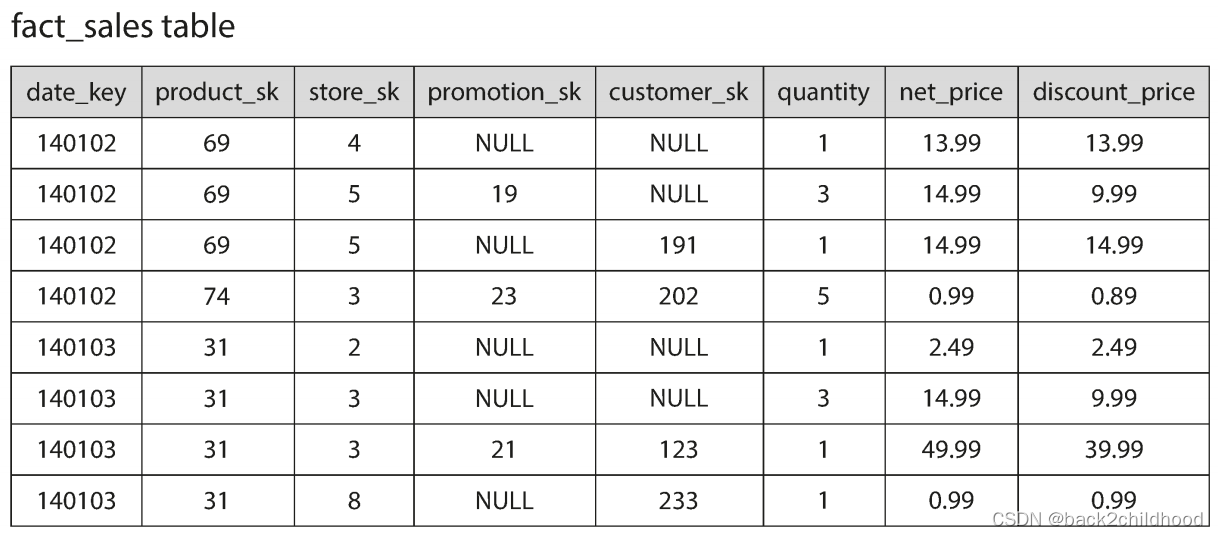
In a typical data warehouse, tables are often very wide: fact tables often have over 100
columns, sometimes several hundred.

Column-Oriented Storage
If we want to analyze whether people are more inclined to buy fresh fruit or candy, depending on the day of the week. It only needs access to three columns of the fact_sales table:daate_key, produck_sk, and quantity. The query ignores all other columns.
But in a row-oriented storage engine still needs to load all of those rows from disk to memory, parse them, and filter out those that don’t meet the required conditions.
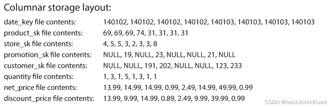
The idea behind column-oriented storage is simple: don’t store all the values from one row together, but store all the values from each column together instead. If each column is stored in a separate file, a query only needs to read and parse those columns that are used in that query, which can save a lot of work.
Column Compression
Take a look at the sequences of values for each column, they look quite repetitive, the following are some approaches for compression.
One technique that is particularly effective in data warehouses is bitmap encoding.
But if the data is bigger, there will be a lot of zeros in most of the bitmaps (we say that they are sparse). In that case, the bitmaps can additionally be run-length encoded.

Bitmap indexes such as these are well suited for the kinds of queries that are common in a data warehouse.
WHERE product_sk IN (30, 68, 69)
Just need to load the three bitmaps for product_sk = 30, 68, 69 and calculate the bitwise OR of the three bitmaps.
Column-oriented storage and column families
Memory bandwidth and vectorized processing
Sort Order in Column Storage
The data needs to be sorted an entire row at a time, even though it is stored by column.
- Advantages:
- help with compression of columns. If the primary sort column does not have many distinct values, then after sorting, it will have long sequences where the same value is repeated many times in a row.
- That will help queries that need to group or filter sales by product within a certain date range.
Several different sort orders
The row-oriented store keeps every row in one place(in a heap file or a clustered index), and secondary indexes just contain pointers to the matching rows. In a column store, there normally aren’t any pointers to data elsewhere, only columns containing values.
Writing to Column-Oriented Storage
- If you wanted to insert a row in the middle of a sorted table, you would most likely have to rewrite all the column files.
- We can use LSM-tree to solve this problem: all writes first go to an in-memory store, where they are added to a sorted structure and prepared for writing to disk. Queries need to examine both the column data on disk and the recent writes in memory and combine the two.
Aggregation: Data Cubes and Materialized Views
Except for column-oriented storage, another aspect of data warehouses is materialized aggregates. As we all know, there are many aggregate functions in SQL, such as COUNT, SUM, MIN, etc. If the same aggregates are used by many different queries, we can cache the counts or sums that queries use most often. This cache is called materialized view.
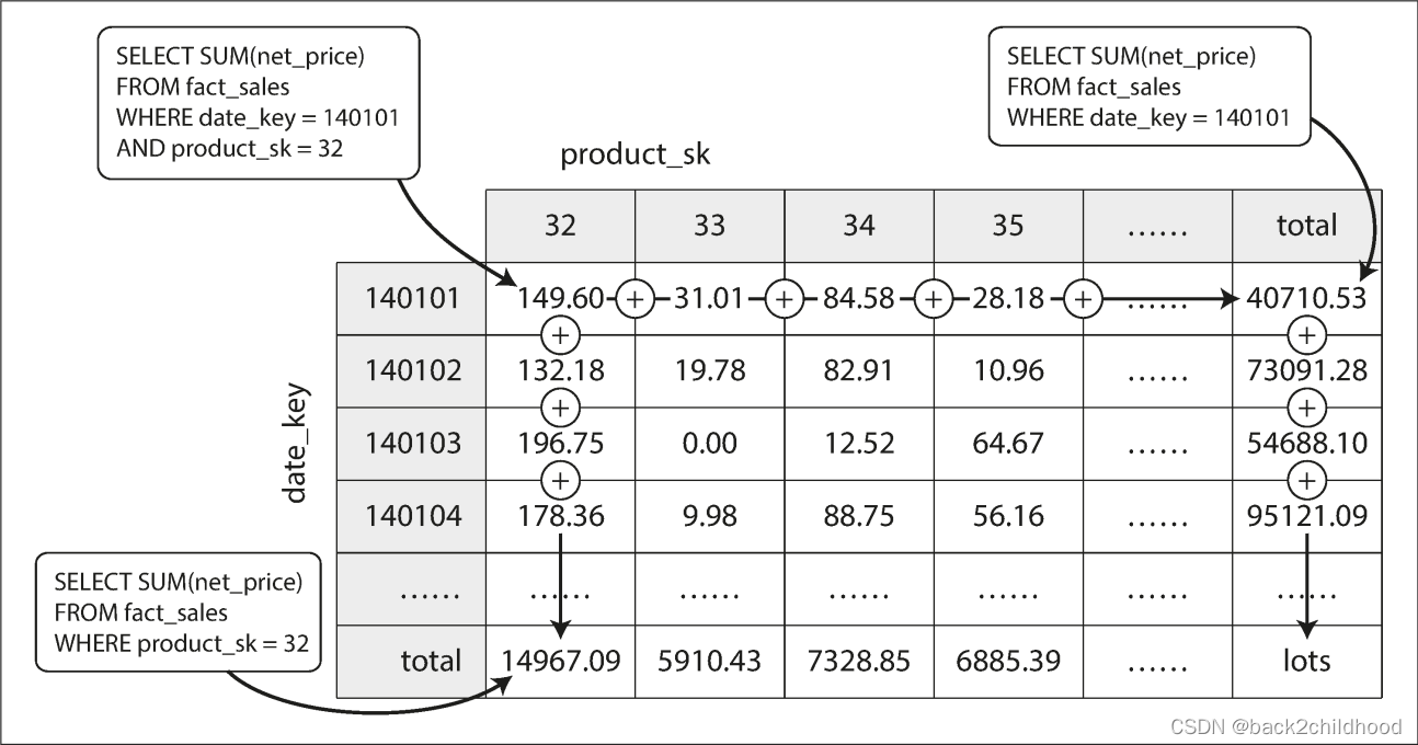
The advantage of a materialized data cube is that certain queries become very fast because they have effectively been precomputed.
The disadvantage is that a data cube doesn’t have the same flexibility as querying the raw data.
Summary
On a high level, we saw that storage engines fall into two broad categories: those optimized for transaction processing (OLTP), and those optimized for analytics (OLAP). There are big differences between the access patterns in those use cases:
- OLTP systems are typically user-facing, which means that they may see a huge volume of requests. In order to handle the load, applications usually only touch a small number of records in each query. The application requests records using some kind of key, and the storage engine uses an index to find the data for the requested key. Disk seek time is often the bottleneck here.
- OLAP and Data warehouses are less well known, because they are primarily used by business analysts, not by end users. They handle a much lower volume of queries than OLTP systems, but each query is typically very demanding, requiring many millions of records to be scanned in a short time. Disk bandwidth (not seek time) is often the bottleneck here, and
column-oriented storageis an increasingly popular solution for this kind of workload.
On the OLTP side, we saw storage engines from two main schools of thought:
- The log-structured school, which only permits appending to files and deleting obsolete files, but never updates a file that has been written. Bitcask, SSTables, LSM-trees, LevelDB, Cassandra, HBase, Lucene, and others belong to this group.
- The update-in-place school, which treats the disk as a set of fixed-size pages that can be overwritten. B-trees are the biggest example of this philosophy, being used in all major relational databases and also many nonrelational ones.


 100
100


 被折叠的 条评论
为什么被折叠?
被折叠的 条评论
为什么被折叠?
 到【灌水乐园】发言


