


一个快速上手各项工具的教程
0. 前言
高性能并行计算专业需要学习的东西非常多且杂,本教程会整合本专业需要学习的一些语言,工具来实现一个简单的logistic回归算法(参考机器学习实战第五章),最终达到对数据进行分类的目的。
1. 创建基本环境
在本tutorial中,我们将使用python来做基本的数据处理,使用C/C++,CUDA来实现核心功能,使用git来进行代码版本管理,使用Makefile/CMake对项目编译进行管理。为了最后结果能够正确实现,这里首先使用conda创建一个相同的环境。
conda create -n tutorial python=3.8  # 使用conda创建基本环境
conda activate tutorial  # 激活tutorial
conda install numpy
conda install matplotlib
conda install -c conda-forge pybind11
conda install -c conda-forge cmake
conda deactivate  # 关闭tutorial
这里提供一个数据集的下载地址,同时这个数据集也被保存在服务器上,可以自行下载。
2. logistic回归原理
本节参考了JackCui的博客,大部分内容是直接拷贝过来的,只对公式部分进行了修改,具体内容可查看原文。
Logistic回归是众多分类算法中的一员。通常,Logistic回归用于二分类问题,例如预测明天是否会下雨。当然它也可以用于多分类问题,不过为了简单起见,本文暂先讨论二分类问题。首先,让我们来了解一下,什么是Logistic回归。
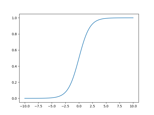
在具体讲解Logistic回归之前,我们首先来认识一个函数sigmoid,它的函数形式是
g
(
z
)
=
1
1
+
e
−
z
g(z) = \frac{1}{1+e^{-z}}
g(z)=1+e−z1,函数大致长下面这样。函数的值在0处等于0.5,此后越往x轴正半轴,值越接近1,越往x轴负半轴,值越接近0。
当前z是一个标量,我们将其拓展为一个向量,则会得到logistic函数,它的函数形式为 h θ ( x ) = g ( θ T x ) = 1 1 + e − θ T x h_{\theta}(x) = g(\theta^{T}x)=\frac{1}{1+e-{\theta^{T}x}} hθ(x)=g(θTx)=1+e−θTx1。其中θ是参数列向量(要求解的),x是样本列向量(给定的数据集)。θ^T表示θ的转置。g(z)函数实现了任意实数到[0,1]的映射,这样我们的数据集([x0,x1,…,xn]),不管是大于1或者小于0,都可以映射到[0,1]区间进行分类。hθ(x)给出了输出为1的概率。比如当hθ(x)=0.7,那么说明有70%的概率输出为1。输出为0的概率是输出为1的补集,也就是30%。
如果我们有合适的参数列向量θ(
[
θ
0
,
θ
1
,
⋯
,
θ
n
]
T
[θ_0,θ_1,\cdots,θ_n]^T
[θ0,θ1,⋯,θn]T),以及样本列向量x([
x
0
,
x
1
,
⋯
,
x
n
x_0,x_1,\cdots,x_n
x0,x1,⋯,xn]),那么我们对样本x分类就可以通过上述公式计算出一个概率,如果这个概率大于0.5,我们就可以说样本是正样本,否则样本是负样本。根据sigmoid函数的特性,我们可以做出如下的假设:
P
(
y
=
1
∣
x
;
θ
)
=
h
θ
(
x
)
P
(
y
=
0
∣
x
;
θ
)
=
1
−
h
θ
(
x
)
P(y=1|x;\theta)=h_{\theta}(x) \\ P(y=0|x;\theta) = 1-h_{\theta}(x)
P(y=1∣x;θ)=hθ(x)P(y=0∣x;θ)=1−hθ(x)
式即为在已知样本x和参数θ的情况下,样本x属性正样本(y=1)和负样本(y=0)的条件概率。理想状态下,根据上述公式,求出各个点的概率均为1,也就是完全分类都正确。但是考虑到实际情况,样本点的概率越接近于1,其分类效果越好。比如一个样本属于正样本的概率为0.51,那么我们就可以说明这个样本属于正样本。另一个样本属于正样本的概率为0.99,那么我们也可以说明这个样本属于正样本。但是显然,第二个样本概率更高,更具说服力。我们可以把上述两个概率公式合二为一:
L
o
s
s
(
h
θ
(
x
)
,
y
)
=
h
θ
(
x
)
y
(
1
−
h
θ
(
x
)
)
(
1
−
y
)
Loss(h_{\theta}(x),y)=h_{\theta}(x)^y(1-h_{\theta}(x))^{(1-y)}
Loss(hθ(x),y)=hθ(x)y(1−hθ(x))(1−y)
合并出来的Loss,我们称之为损失函数(Loss Function)。当y等于1时,(1-y)项(第二项)为0;当y等于0时,y项(第一项)为0。为s了简化问题,我们对整个表达式求对数,(将指数问题对数化是处理数学问题常见的方法):
L
o
s
s
(
h
θ
(
x
)
,
y
)
=
y
log
h
θ
(
x
)
+
(
1
−
y
)
log
(
1
−
h
θ
(
x
)
)
Loss(h_{\theta}(x),y)=y\log h_{\theta}(x)+(1-y)\log (1-h_{\theta}(x))
Loss(hθ(x),y)=yloghθ(x)+(1−y)log(1−hθ(x))
这个损失函数,是对于一个样本而言的。给定一个样本,我们就可以通过这个损失函数求出,样本所属类别的概率,而这个概率越大越好,所以也就是求解这个损失函数的最大值。既然概率出来了,那么最大似然估计也该出场了。假定样本与样本之间相互独立,那么整个样本集生成的概率即为所有样本生成概率的乘积,便可得到如下公式:
J
(
θ
)
=
∑
i
=
1
m
[
y
(
i
)
log
h
θ
(
x
(
i
)
)
+
(
1
−
y
(
i
)
)
log
(
1
−
h
θ
(
x
(
i
)
)
)
]
J(\theta)=\sum_{i=1}^{m}[y^{(i)}\log h_{\theta}(x^{(i)})+(1-y^{(i)})\log (1-h_{\theta}(x^{(i)}))]
J(θ)=i=1∑m[y(i)loghθ(x(i))+(1−y(i))log(1−hθ(x(i)))]
其中,m为样本的总数,y(i)表示第i个样本的类别,x(i)表示第i个样本,需要注意的是θ是多维向量,x(i)也是多维向量。
综上所述,满足J(θ)的最大的θ值即是我们需要求解的模型。为了求解使J(θ)最大的θ值呢,我们还需要使用梯度下降算法(梯度下降法内容非常基础,这里不再赘述,只要会牛顿迭代法就能理解梯度下降法的思想)。
x
i
+
1
=
x
i
−
α
∂
f
x
i
x
i
θ
j
:
=
θ
j
−
α
∂
J
(
θ
j
)
θ
j
x_{i+1} = x_{i}-\alpha\frac{\partial f{x_i}}{x_i} \\ \theta_{j}:=\theta_{j}-\alpha\frac{\partial {J(\theta_j)}}{\theta_j}
xi+1=xi−αxi∂fxiθj:=θj−αθj∂J(θj)
现在我们只要求出J(θ)的偏导,就可以利用梯度上升算法,求解J(θ)的极大值了。求解如下:
∂
∂
θ
j
J
(
θ
)
=
∂
J
(
θ
)
∂
g
(
θ
T
x
)
∗
∂
g
(
θ
T
x
)
∂
θ
T
x
∗
∂
θ
T
x
∂
θ
j
\frac{\partial}{\partial \theta_j}J(\theta)=\frac{\partial J(\theta)}{\partial g(\theta^Tx)}*\frac{\partial g(\theta^Tx)}{\partial\theta^Tx} * \frac{\partial\theta^Tx}{\partial\theta_j}
∂θj∂J(θ)=∂g(θTx)∂J(θ)∗∂θTx∂g(θTx)∗∂θj∂θTx
其中:
∂
J
(
θ
)
∂
g
(
θ
T
x
)
=
y
∗
1
g
(
θ
T
x
)
+
(
y
−
1
)
∗
1
1
−
g
(
θ
T
x
)
\frac{\partial J(\theta)}{\partial g(\theta^Tx)}=y*\frac{1}{g(\theta^Tx)}+(y-1)*\frac{1}{1-g(\theta^Tx)}
∂g(θTx)∂J(θ)=y∗g(θTx)1+(y−1)∗1−g(θTx)1
已知:
g
′
(
z
)
=
d
d
z
1
1
+
e
(
−
z
)
=
g
(
z
)
(
1
−
g
(
z
)
)
g'(z) = \frac{d}{dz}\frac{1}{1+ e ^{(-z)}}=g(z)(1-g(z))
g′(z)=dzd1+e(−z)1=g(z)(1−g(z))
则:
∂
g
(
θ
T
x
)
∂
θ
T
x
=
g
(
θ
T
x
)
(
1
−
g
(
θ
T
x
)
)
\frac{\partial g(\theta^Tx)}{\partial\theta^Tx}=g(\theta^Tx)(1-g(\theta^Tx))
∂θTx∂g(θTx)=g(θTx)(1−g(θTx))
接下来,就剩下第三部分:
∂
θ
T
x
∂
θ
j
=
∂
J
(
θ
1
x
1
+
θ
2
x
2
+
⋯
+
θ
n
x
n
)
∂
θ
j
=
x
j
\frac{\partial\theta^Tx}{\partial\theta_j} = \frac{\partial J(\theta_1x_1+\theta_2x_2+\cdots+\theta_nx_n)}{\partial \theta_j}=x_j
∂θj∂θTx=∂θj∂J(θ1x1+θ2x2+⋯+θnxn)=xj
综上所述:
θ
j
:
=
θ
j
−
α
∑
i
=
1
m
(
y
(
i
)
−
h
θ
(
x
(
i
)
)
)
x
j
(
i
)
\theta_j:=\theta_j - \alpha\sum_{i=1}^{m}(y^{(i)}-h_\theta(x^{(i)}))x_j^{(i)}
θj:=θj−αi=1∑m(y(i)−hθ(x(i)))xj(i)
3. python3实战
本节你将学习git的基本用法,使用git来管理项目;学习python,使用numpy来进行科学计算,使用matplotlib来进行结果展示。
从本节开始,后续每一节都会写代码,并且是在上一节的基础上添加各种特性,因此这里我们使用git来进行项目管理。首先创建一个叫tutorial的文件夹,然后进入该文件夹。
mkdir tutorial  # 创建文件夹
cd tutorial  # 进入文件夹
接下来要使用git对整个文件夹进行初始化,以便后续管理。
git init
接下来的命令是用于配置git的,你可以选择跳过。
git config --global user.name "Zhang San"           # 你的名字
git config --global user.email "zhangsan@foo.com"   # 你的email
git config --global core.editor vim                 # 你最常用的editor
git config --global color.ui true
设置完成之后下面创建一个README.md文件用于说明仓库的功能,这里我直接在README中添加一句很简单的话作为仓库的说明。接下来使用git add指令将文件放置在缓冲区,然后使用git commit为当前提交添加说明,然后再与远程仓库相关联(这里你需要提前在github上创建一个仓库,然后使用仓库的链接替换这里的网址),最后使用git push将README.md提交至远程仓库。
touch README.md && echo "This is a tutorial" >> README.md
git add README.md
git commit -m "first commit"
git remote add origin https://github.com/xxx/tutorail.git
git push -u origin "master"
至此已经完成了所有的准备工作,下面我们将创建一个新的分支,用python实现logistic回归。
git checkout -b python3
使用上述指令会创建一个新的名为python3的分支,在当前分支下你将会看到一个从master分支拷贝过来的README文件。接下来我们开始编写代码,由于python代码过于简单,这里直接提供,不做过多的解释。
import matplotlib.pyplot as plt
import numpy as np

def loadDataSet():
    dataMat = []
    labelMat = []
    fr = open('testSet.txt')
    for line in fr.readlines():
        lineArr = line.strip().split()
        dataMat.append([1.0, float(lineArr[0]), float(lineArr[1])])
        labelMat.append(int(lineArr[2]))
    fr.close()
    return dataMat, labelMat

def sigmoid(inX):
    return 1.0 / (1 + np.exp(-inX))

def gradAscent(dataMatIn, classLabels):
    dataMatrix = np.mat(dataMatIn)
    labelMat = np.mat(classLabels).transpose()
    m, n = np.shape(dataMatrix)
    alpha = 0.001
    maxCycles = 500
    weights = np.ones((n,1))
    for k in range(maxCycles):
        h = sigmoid(dataMatrix * weights)
        error = labelMat - h
        weights = weights + alpha * dataMatrix.transpose() * error
    return weights.getA()

def plotBestFit(weights):
    dataMat, labelMat = loadDataSet()
    dataArr = np.array(dataMat)
    n = np.shape(dataMat)[0]
    xcord1 = []; ycord1 = []
    xcord2 = []; ycord2 = []
    for i in range(n):
        if int(labelMat[i]) == 1:
            xcord1.append(dataArr[i,1]); ycord1.append(dataArr[i,2])
        else:
            xcord2.append(dataArr[i,1]); ycord2.append(dataArr[i,2])
    fig = plt.figure()
    ax = fig.add_subplot(111)
    ax.scatter(xcord1, ycord1, s = 20, c = 'red', marker = 's',alpha=.5)
    ax.scatter(xcord2, ycord2, s = 20, c = 'green',alpha=.5)
    x = np.arange(-3.0, 3.0, 0.1)
    y = (-weights[0] - weights[1] * x) / weights[2]
    ax.plot(x, y)
    plt.title('BestFit')
    plt.xlabel('X1'); plt.ylabel('X2')
    plt.savefig('result.png')
    plt.show()

if __name__ == '__main__':
    dataMat, labelMat = loadDataSet()
    weights = gradAscent(dataMat, labelMat)
    plotBestFit(weights)
同时我们将下载的数据集拷贝到当前的文件夹,然后使用python3 logistic.py运行脚本。
# 注意,这里需要将目录和文件名换成你自己的
cp ~/testSet.txt .
python3 logistic.py
如果程序正确运行,你将会看到下面的图片,并且在当前文件夹下还会生成一张名为result.png的图片。 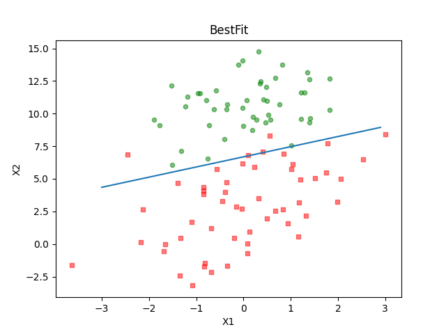
至此我们已经完成了使用python实现logistic算法,现在我们可以把它push到远程仓库。
git add .
git commit -m "python3 logistic"
git remote add origin https://github.com/xxx/tutorail.git
git push -u origin "python3"
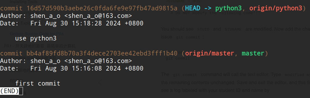
这个时候我们可以使用git log查看我们的提交记录。该log会详细显示,提交人是谁,在什么时候提交的代码,以及提交时添加的备注。
如果此时你使用git checkout master切回到master分支,你将会发现刚才我们写的代码,生成的图片,以及拷贝的数据集都不见了。不用惊慌,这就是git的特性,每个分支之间是相互独立不影响的,此时再使用git checkout python3就可以切换回python3分支,此时可以看到所有的文件又全部恢复了。
4. C/C++实战
本节你将学习Makefile的基本语法,modern c++的基本语法,以及编译的基本方法。
本节我们将使用C++实现logistic算法,相较于python,C++的代码会比较繁琐,包括数据读取,预处理,以及向量矩阵乘都得我们自行实现。由于需要实现的功能较多,这里我们并不将所有的代码放在一个文件中,而是按功能将其拆分成多个文件,最后为了降低编译的难度,这里会提供一个Makefile,这使得每次编译只需要输入make即可。整体的代码框架如下所示:
.
├── grad_ascend.cpp
├── grad_ascend.hpp
├── load_data.cpp
├── load_data.hpp
├── main.cpp
├── Makefile
├── README.md
└── testSet.txt
其中load_data.cpp主要用于从文本文件中读取数据,grad_ascend.cpp实现了logistic回归主要的步骤,main.cpp负责使用load_data.cpp和grad_ascend.cpp提供的函数实现整体的功能,最终会输出拟合得到的
θ
\theta
θ,代码如下所示:
/* load_data.hpp*/
#ifndef _LOAD_DATA_H
#define _LOAD_DATA_H
#include <vector>
#include <string>
void readData(const std::string &filename, std::vector<std::vector<double>> &X,
              std::vector<double> &y);
#endif //LOAD_DATA_H

/* =================================================== */

/* load_data.cpp */
#include <fstream>
#include <iostream>
#include <sstream>
#include "load_data.hpp"

void readData(const std::string &filename, std::vector<std::vector<double>> &X,
              std::vector<double> &y) {
  std::ifstream file(filename);
  if (!file.is_open()) {
    std::cerr << "无法打开文件!" << std::endl;
    return;
  }

  std::string line;
  while (std::getline(file, line)) {
    std::istringstream iss(line);
    std::vector<double> row;
    double value;

    row.push_back(1.0); // 偏置项
    while (iss >> value) {
      row.push_back(value);
    }

    y.push_back(row.back());
    row.pop_back();

    X.push_back(row);
  }

  file.close();
}

#ifdef _LOAD_DATA_MAIN
int main() {
  std::vector<std::vector<double>> X;
  std::vector<double> y;

  readData("testSet.txt", X, y);
  std::cout << "X:" << std::endl;
  for (const auto &row : X) {
    for (const auto &val : row) {
      std::cout << val << " ";
    }
    std::cout << std::endl;
  }

  std::cout << "y:" << std::endl;
  for (const auto &val : y) {
    std::cout << val << std::endl;
  }

  return 0;
}
#endif


/* =================================================== */
/* grad_ascend.hpp */
#ifndef _GRAD_ASCEND_H
#define _GRAD_ASCEND_H

double sigmoid(double x);
void mat_vec_mul(std::vector<std::vector<double>> &X, std::vector<double> &w,
                 std::vector<double> &res);
std::vector<double> grad_ascend(std::vector<std::vector<double>> X,
                               std::vector<double> y);
#endif //GRAD_ASCEND_H

/* =================================================== */
/* grad_ascend.cpp */
#include <cmath>
#include <iostream>
#include <vector>
#include "grad_ascend.hpp"

double sigmoid(double x) { return 1.0 / (1.0 + exp(-x)); }

void mat_vec_mul(std::vector<std::vector<double>> &X, std::vector<double> &w,
                 std::vector<double> &res) {
  int m = X.size();
  int n = X[0].size();
  for (int i = 0; i < m; i++) {
    res[i] = 0.0;
    for (int j = 0; j < n; j++) {
      res[i] += X[i][j] * w[j];
    }
  }
}

std::vector<double> grad_ascend(std::vector<std::vector<double>> X,
                               std::vector<double> y) {
  int m = X.size();
  int n = X[0].size();
  double alpha = 0.001;
  int max_iter = 500;
  std::vector<double> w(n, 0.0);
  for (int i = 0; i < max_iter; i++) {
    std::vector<double> h(m, 0.0);
    std::vector<double> err(m, 0.0);
    mat_vec_mul(X, w, h);
    for (int j = 0; j < m; j++) {
      h[j] = sigmoid(h[j]);
      err[j] = y[j] - h[j];
    }

    std::vector<double> grad(n, 0.0);
    for (int j = 0; j < n; j++) {
      for (int k = 0; k < m; k++) {
        grad[j] += X[k][j] * err[k];
      }
      w[j] += alpha * grad[j];
    }
  }
  return w;
}

/* =================================================== */
/* main.cpp */
#include <iostream>
#include "load_data.hpp"
#include "grad_ascend.hpp"

int main() {
  std::vector<std::vector<double>> X;
  std::vector<double> y;

  readData("testSet.txt", X, y);

  std::vector<double> w = grad_ascend(X, y);
  std::cout << "w: ";
  for (int i = 0; i < w.size(); i++) {
    std::cout << w[i] << " ";
  }
  std::cout << std::endl;
  return 0;

}
可以看到在load_data.cpp的结尾处我们添加了一个条件编译选项_LOAD_DATA_MAIN ,这种方法在多文件联合编译的时候是很有用的,它的主要功能是测试当前模块内的函数功能是否正确实现,并且可以单独测试。如果想要进行测试,我们只需要单独编译着一个文件即可。
g++ -D_LOAD_DATA_MAIN load_data.cpp -o load_data
Makefile的内容如下所示:
CPPFLAGS= -O2 -std=c++11 # 可选参数 -Wall -Werror
INCLUDES=
OBJS= main.o grad_ascend.o load_data.o
PROG= logistic
LIBS= -lm

$(PROG): $(OBJS)
	g++ $(CPPFLAGS) $(INCLUDES) -o $(PROG) $(OBJS)

main.o: main.cpp
	g++ $(CPPFLAGS) $(INCLUDES) -c main.cpp

grad_ascend.o: grad_ascend.cpp
	g++ $(CPPFLAGS) $(INCLUDES) -c grad_ascend.cpp

load_data.o: load_data.cpp
	g++ $(CPPFLAGS) $(INCLUDES) -c load_data.cpp

.PHONY: clean
clean:
	rm -f $(PROG) $(OBJS)
Makefile的书写规则其实非常简单,就只包含两个部分,一个是依赖关系,一个是生成目标的方法。只要记住这两个部分基本上就能写出正确的Makfile。同时我们也可以看到,虽然源文件很少,但是Makefile也要写一大堆,这就是Makefile的弊端,尤其是在面对大型项目时,写Makefile其实是一件不太容易的事,因此后面的章节中我们还会提供CMake的tutorial,体验更加快捷的方法。
5. python, C/C++, pybind11
本节你将学习CMake的基本语法,pybind的基本用法,以及如何使用pybind将python代码中的核心部分使用C/C++进行改写并加速。
通过三四两节我们可以看到,python在文件和图像处理方面相较于C/C++具有较大的优势,而C/C++在运行效率上天然比python更高。因此我们会有一个想法就是能否对python代码中的核心步骤使用C/C++进行改写,python代码在执行到这一部分时直接调用C/C++实现的功能,这样整个程序的运行效率就会高一个档次。要实现这个功能我们需要使用pybind这个库。
Pybind11是一个轻量级的只有头文件的库,它在 Python 中公开C++ 类型,反之亦然,主要用于创建现有C++代码的Python 绑定。它的目标和语法类似于由David Abrahams开发的优秀的Boost的Python库: 通过使用编译时自省来推断类型信息,从而最小化传统扩展模块中的样板代码。
conda install -c conda-forge pybind11 # 在环境中使用conda安装pybind11
相较于纯使用python实现的logistic,我们这里只使用它处理文件和画图部分的代码。
import matplotlib.pyplot as plt
import numpy as np
from grad_ascend import gradAscent

def loadDataSet():
    dataMat = []
    labelMat = []
    fr = open('testSet.txt')
    for line in fr.readlines():
        lineArr = line.strip().split()
        dataMat.append([1.0, float(lineArr[0]), float(lineArr[1])])
        labelMat.append(int(lineArr[2]))
    fr.close()
    return dataMat, labelMat

def plotBestFit(weights):
    dataMat, labelMat = loadDataSet()
    dataArr = np.array(dataMat)
    n = np.shape(dataMat)[0]
    xcord1 = []; ycord1 = []
    xcord2 = []; ycord2 = []
    for i in range(n):
        if int(labelMat[i]) == 1:
            xcord1.append(dataArr[i,1]); ycord1.append(dataArr[i,2])
        else:
            xcord2.append(dataArr[i,1]); ycord2.append(dataArr[i,2])
    fig = plt.figure()
    ax = fig.add_subplot(111)
    ax.scatter(xcord1, ycord1, s = 20, c = 'red', marker = 's',alpha=.5)
    ax.scatter(xcord2, ycord2, s = 20, c = 'green',alpha=.5)
    x = np.arange(-3.0, 3.0, 0.1)
    y = (-weights[0] - weights[1] * x) / weights[2]
    ax.plot(x, y)
    plt.title('BestFit')
    plt.xlabel('X1'); plt.ylabel('X2')
    plt.savefig('result.png')
    plt.show()

if __name__ == '__main__':
    dataMat, labelMat = loadDataSet()
    weights = gradAscent(dataMat, labelMat)
    plotBestFit(weights)
接下来实现gradAscent的代码文件我们按照惯例将其放在src文件夹下。
mkdir src
touch grad_ascend.cpp
grad_ascend.cpp文件中存储了gradAscent函数的具体实现方法。
#include <pybind11/numpy.h>
#include <pybind11/pybind11.h>
#include <pybind11/stl.h>

#include <cmath>
#include <iostream>
#include <vector>

double sigmoid(double x) { return 1.0 / (1.0 + exp(-x)); }

void mat_vec_mul(std::vector<std::vector<double>> &X, std::vector<double> &w,
                 std::vector<double> &res) {
  int m = X.size();
  int n = X[0].size();
  for (int i = 0; i < m; i++) {
    res[i] = 0.0;
    for (int j = 0; j < n; j++) {
      res[i] += X[i][j] * w[j];
    }
  }
}

std::vector<double> gradAscend(std::vector<std::vector<double>> X,
                                std::vector<double> y) {
  int m = X.size();
  int n = X[0].size();
  double alpha = 0.001;
  int max_iter = 500;
  std::vector<double> w(n, 0.0);
  for (int i = 0; i < max_iter; i++) {
    std::vector<double> h(m, 0.0);
    std::vector<double> err(m, 0.0);
    mat_vec_mul(X, w, h);
    for (int j = 0; j < m; j++) {
      h[j] = sigmoid(h[j]);
      err[j] = y[j] - h[j];
    }

    std::vector<double> grad(n, 0.0);
    for (int j = 0; j < n; j++) {
      for (int k = 0; k < m; k++) {
        grad[j] += X[k][j] * err[k];
      }
      w[j] += alpha * grad[j];
    }
  }
  return w;
}

PYBIND11_MODULE(grad_ascend, m) {
  m.doc() = "pybind11 grad_ascend plugin"; // optional module docstring
  m.def("gradAscend", &gradAscend, "A function to do gradient ascend");
}
相较于C/C++实现的部分,我们多了PYBIND11_MODULE这个函数,而这个函数的功能正是将cpp实现的gradAscend函数传递给python代码,并且将名字也定义为gradAscend。实际上pybind11干的事情就是将我们实现的cpp编译成一个动态链接库,这样python脚本在运行时碰到cpp实现的函数直接从动态链接库调用即可。怎么将C/C++代码编译成动态链接库又是一个问题,实际上使用g++就能完成,但是在大型项目中要处理的文件很多,一般我们使用CMake来进行管理。
g++ -O3 -Wall -shared -std=c++11 -fPIC $(python3 -m pybind11 --includes) grad_ascend.cpp -o grad_ascend
这里仍旧提供一个基本的命令,如果后续想要了解更多可以自行查资料(上一节关于gcc的参考书中有相关章节)。本节我们使用更加通用的CMake来作为示例:
cmake_minimum_required(VERSION 3.15)

if (POLICY CMP0148)
    cmake_policy(SET CMP0148 OLD)
endif()

project(grad_ascend C CXX)

# find correct version of Python
execute_process(COMMAND python3-config --prefix
  OUTPUT_VARIABLE Python_ROOT_DIR)
find_package(PythonInterp COMPONENTS Development Interpreter REQUIRED)
include_directories(${Python_INCLUDE_DIRS})

# find pybind11
find_package(pybind11 REQUIRED)

# Include Python and pybind11 headers
include_directories(${Python3_INCLUDE_DIRS})
include_directories(${pybind11_INCLUDE_DIRS})

# Add the module library
add_library(grad_ascend MODULE src/grad_ascend.cpp)
target_link_libraries(grad_ascend PRIVATE pybind11::module)

set_target_properties(grad_ascend
  PROPERTIES
  LIBRARY_OUTPUT_DIRECTORY ${CMAKE_CURRENT_SOURCE_DIR}
  CXX_VISIBILITY_PRESET "hidden"
  PREFIX ""
)
CMake的语法其实跟搭积木很相似,每个函数执行一个功能,我们需要什么、功能就去它提供的函数中找相应的API,最后将整块积木拼完,也就完成了整个项目。这里我们的目的是使用pybind11头文件来关联C/C++和python,因此我们首先得找到pybind11,并将相应的头文件引入到项目中。有了基础的依赖库之后我们就可以使用编译器将源码编程成动态链接库了,这里只需要注意CMake在将源码编译成库的时候会自动在库名前加上lib这个前缀,因此我们需要设置其属性,去掉这个前缀。CMake整体的逻辑非常清晰,熟练使用CMake可以大幅降低编译和项目管理的难度。
cmake -Bbuild . && cd build
make
使用上述指令可以轻松在build文件夹下完成对cpp文件的编译,最终在当前目录下生成得到的动态链接库,最后我们使用python logistic.py执行脚本,也会成功得到result.png。
6. OpenMP
本节你将学习OpenMP的基本用法,以及CMake寻找OpenMP的方法。
OpenMP实际上非常简单,这里本来并不想单独用一节来讲解。但是考虑到前后小节逻辑的整体性,本节会介绍OpenMP的基本用法。相较于第五节的cpp代码,本节的代码只多添加了几句#pragma omp parallel for,但是正是这几句却可以大幅提高程序的效率。
#include <pybind11/numpy.h>
#include <pybind11/pybind11.h>
#include <pybind11/stl.h>

#include <cmath>
#include <iostream>
#include <vector>
#include <omp.h>

double sigmoid(double x) { return 1.0 / (1.0 + exp(-x)); }

void mat_vec_mul(std::vector<std::vector<double>> &X, std::vector<double> &w,
                 std::vector<double> &res) {
  int m = X.size();
  int n = X[0].size();
#pragma omp parallel for
  for (int i = 0; i < m; i++) {
    res[i] = 0.0;
    for (int j = 0; j < n; j++) {
      res[i] += X[i][j] * w[j];
    }
  }
}

std::vector<double> gradAscend(std::vector<std::vector<double>> X,
                                std::vector<double> y) {
  int m = X.size();
  int n = X[0].size();
  double alpha = 0.001;
  int max_iter = 500;
  std::vector<double> w(n, 0.0);
  for (int i = 0; i < max_iter; i++) {
    std::vector<double> h(m, 0.0);
    std::vector<double> err(m, 0.0);
    mat_vec_mul(X, w, h);
#pragma omp parallel for
    for (int j = 0; j < m; j++) {
      h[j] = sigmoid(h[j]);
      err[j] = y[j] - h[j];
    }

    std::vector<double> grad(n, 0.0);
#pragma omp parallel for
    for (int j = 0; j < n; j++) {
      for (int k = 0; k < m; k++) {
        grad[j] += X[k][j] * err[k];
      }
      w[j] += alpha * grad[j];
    }
  }
  return w;
}

PYBIND11_MODULE(grad_ascend, m) {
  m.doc() = "pybind11 grad_ascend plugin"; // optional module docstring
  m.def("gradAscend", &gradAscend, "A function to do gradient ascend");
}
OpenMP允许程序员使用编译指导语言来对代码块进行“标注”,让编译器知道哪一块代码存在潜在的可并行性,以及如何进行并行。这样的方式大大降低了程序员的编程压力,使得程序员只需要在原来代码的基础上添加几句话就可以让程序得到不俗的加速。本节只展示了for这一指导语句,更多的内容请自行查看前文的tutorial。
cmake_minimum_required(VERSION 3.15)

if (POLICY CMP0148)
    cmake_policy(SET CMP0148 OLD)
endif()

project(grad_ascend C CXX)

# find correct version of Python
execute_process(COMMAND python3-config --prefix
  OUTPUT_VARIABLE Python_ROOT_DIR)
find_package(PythonInterp COMPONENTS Development Interpreter REQUIRED)
include_directories(${Python_INCLUDE_DIRS})

# find pybind11
find_package(pybind11 REQUIRED)

# Include Python and pybind11 headers
include_directories(${Python3_INCLUDE_DIRS})
include_directories(${pybind11_INCLUDE_DIRS})

# find openmp
find_package(OpenMP REQUIRED)

# Add the module library
add_library(grad_ascend MODULE src/grad_ascend.cpp)
target_link_libraries(grad_ascend PRIVATE pybind11::module OpenMP::OpenMP_CXX)

set_target_properties(grad_ascend
  PROPERTIES
  LIBRARY_OUTPUT_DIRECTORY ${CMAKE_CURRENT_SOURCE_DIR}
  CXX_VISIBILITY_PRESET "hidden"
  PREFIX ""
)
CMakeLists.txt中其实也只修改了两个地方:1️⃣ 增加了寻找OpenMP的方法;2️⃣ 最终的动态链接库链接了OpenMP,其余跟前文完全一致。
7. CUDA
本节你将学习CUDA的基本语法,CMake条件编译,以及如何编译cuda代码。
上一节我们使用OpenMP对cpp核心代码进行了加速,但是CPU的算力是一定的,而且远远小于同时代的GPU,在处理大规模的数据时我们如果能够使用GPU对数据进行处理,那么将大大提高程序的效率。本节我们的任务就是将上一节的cpp代码修改成cuda代码并将其成功部署在GPU上,使其正确运行。我们接下来要做的事情其实跟深度学习中的算子开发是一个概念:都是将算法的核心步骤搬到GPU上工作。
#include <cuda_runtime.h>
#include <pybind11/numpy.h>
#include <pybind11/pybind11.h>
#include <pybind11/stl.h>

#include <cmath>
#include <iostream>
#include <vector>

#define BLOCK_SIZE 256

// CUDA sigmoid function
__device__ double sigmoid(double x) { return 1.0 / (1.0 + exp(-x)); }

// CUDA kernel for matrix-vector multiplication
__global__ void mat_vec_mul(double *X, double *w, double *h, int m, int n) {
  int row = blockIdx.x * blockDim.x + threadIdx.x;
  if (row < m) {
    double result = 0.0;
    for (int j = 0; j < n; j++) {
      result += X[row * n + j] * w[j];
    }
    h[row] = sigmoid(result); // Apply sigmoid directly
  }
}

// CUDA kernel for computing the gradient
__global__ void compute_gradient(double *X, double *h, double *y, double *grad,
                                 int m, int n) {
  int tid = blockIdx.x * blockDim.x + threadIdx.x;
  if (tid < n) {
    double sum = 0.0;
    for (int i = 0; i < m; i++) {
      sum += (y[i] - h[i]) * X[i * n + tid];
    }
    grad[tid] = sum;
  }
}

// Host function for gradient ascent
std::vector<double> gradAscend(std::vector<std::vector<double>> &X,
                               std::vector<dou-ble> &y) {
  int m = X.size();
  int n = X[0].size();
  double alpha = 0.001;
  int max_iter = 500;

  // Flatten the 2D vector X for GPU
  std::vector<double> X_flat(m * n);
  for (int i = 0; i < m; i++) {
    for (int j = 0; j < n; j++) {
      X_flat[i * n + j] = X[i][j];
    }
  }

  // Allocate memory on GPU
  double *d_X, *d_w, *d_h, *d_y, *d_grad;
  cudaMalloc(&d_X, m * n * sizeof(double));
  cudaMalloc(&d_w, n * sizeof(double));
  cudaMalloc(&d_h, m * sizeof(double));
  cudaMalloc(&d_y, m * sizeof(double));
  cudaMalloc(&d_grad, n * sizeof(double));

  // Initialize w and copy data to GPU
  std::vector<double> w(n, 0.0);
  cudaMemcpy(d_X, X_flat.data(), m * n * sizeof(double),
             cudaMemcpyHostToDevice);
  cudaMemcpy(d_y, y.data(), m * sizeof(double), cudaMemcpyHostToDevice);
  cudaMemcpy(d_w, w.data(), n * sizeof(double), cudaMemcpyHostToDevice);

  // Start gradient ascent loop
  for (int iter = 0; iter < max_iter; iter++) {
    // Compute h = sigmoid(X * w)
    int num_blocks = (m + BLOCK_SIZE - 1) / BLOCK_SIZE;
    mat_vec_mul<<<num_blocks, BLOCK_SIZE>>>(d_X, d_w, d_h, m, n);

    // Compute gradient
    num_blocks = (n + BLOCK_SIZE - 1) / BLOCK_SIZE;
    compute_gradient<<<num_blocks, BLOCK_SIZE>>>(d_X, d_h, d_y, d_grad, m, n);

    // Update weights
    std::vector<double> grad(n);
    cudaMemcpy(grad.data(), d_grad, n * sizeof(double), cudaMemcpyDeviceToHost);
    for (int j = 0; j < n; j++) {
      w[j] += alpha * grad[j];
    }

    // Copy updated weights back to GPU
    cudaMemcpy(d_w, w.data(), n * sizeof(double), cudaMemcpyHostToDevice);
  }

  // Clean up
  cudaFree(d_X);
  cudaFree(d_w);
  cudaFree(d_h);
  cudaFree(d_y);
  cudaFree(d_grad);

  return w;
}

PYBIND11_MODULE(grad_ascend, m) {
  m.doc() = "pybind11 grad_ascend plugin"; // optional module docstring
  m.def("gradAscend", &gradAscend, "A function to do gradient ascend");
}
CUDA代码的编写其实跟将大象放进冰箱是一个道理,将数据从CPU拷贝至GPU对应打开冰箱门,在GPU上做运算相当于是将大象塞进冰箱,最后将得到的结果拷贝回CPU则对应将冰箱门关上。其中第一步和第三步我们可以看到只是涉及到数据的处理,而最为关键同时也最难的步骤就是“怎么将大象塞进冰箱”。CUDA编程模型是SIMT,即单指令流多线程,我们需要做的是对数据进行分块,然后将每一块的运算都分给对应的线程完成,需要注意的是这里每个线程都要做尽量做相同的事情,否则程序的运行效率会大幅降低,而往往这一步就是最困难的。我们学习CUDA编程,首先并且长期需要学习的就是各个优秀项目中数据分块的方式。
cmake_minimum_required(VERSION 3.15)
if (POLICY CMP0148)
    cmake_policy(SET CMP0148 OLD)
endif()

project(grad_ascend C CXX)
# find correct version of Python
execute_process(COMMAND python3-config --prefix
  OUTPUT_VARIABLE Python_ROOT_DIR)
find_package(PythonInterp COMPONENTS Development Interpreter REQUIRED)
include_directories(${Python_INCLUDE_DIRS})

# find pybind11
find_package(pybind11 REQUIRED)

# Include Python and pybind11 headers
include_directories(${Python3_INCLUDE_DIRS})
include_directories(${pybind11_INCLUDE_DIRS})

find_package(CUDA)
if(CUDA_FOUND)
    # Add the module library with CUDA
    message(STATUS "CUDA found")
    include_directories(SYSTEM ${CUDA_INCLUDE_DIRS})
    list(APPEND LINKER_LIBS ${CUDA_CUDART_LIBRARY})

    execute_process(COMMAND "nvidia-smi" ERROR_QUIET RESULT_VARIABLE NV_RET)
    if(NV_RET EQUAL 0)
        CUDA_SELECT_NVCC_ARCH_FLAGS(ARCH_FLAGS Auto)
    else()
        CUDA_SELECT_NVCC_ARCH_FLAGS(ARCH_FLAGS 3.7)
    endif()

    CUDA_ADD_LIBRARY(grad_ascend MODULE src/grad_ascend.cu OPTIONS ${ARCH_FLAGS})

    # Use PRIVATE to link the libraries
    target_link_libraries(grad_ascend ${LINKER_LIBS})
    pybind11_extension(grad_ascend)
    pybind11_strip(grad_ascend)

else()
    # Add the module library without CUDA
    add_library(grad_ascend MODULE src/grad_ascend.cpp)

    # Use PRIVATE to link the libraries
    target_link_libraries(grad_ascend PRIVATE pybind11::module)
endif()

set_target_properties(grad_ascend
     PROPERTIES
     LIBRARY_OUTPUT_DIRECTORY ${CMAKE_CURRENT_SOURCE_DIR}
     CXX_VISIBILITY_PRESET "hidden"
     PREFIX ""
)
为了保证我们的项目能够在即使是在没有GPU卡的机器上稳定运行,这里也对CMakeLisis.txt进行了修改,增加了条件编译选项:如果在机器上找到了GPU卡我们就编译CUDA版本的动态链接库,如果找不到就编译普通的c++版本。需要注意的是cuda编译使用的nvcc版本需要跟GPU卡的型号适配,此外nvcc还限制了gcc的版本,我们在创建环境时需要务必注意,负责编译会出错。
# e.g. nvcc version = 11.2
conda install -c conda-forge gcc=9
conda install -c conda-forge gxx=9
8. 总结
本教程综合了python,C/C++,CUDA,git,Makefile,CMake,OpenMP,conda,机器学习,gcc/g++,pybind等内容,基本上我们专业需要学习的各种语言,各项工具都有一个基本的介绍,相信读者从头到尾仔细复现一遍会对这些工具以及我们专业需要学习的知识有大致的印象。需要注意的是,tutorial并没有按照说明书那般将每一个细节都说清楚,在运行程序的时候你可能会遇到各种各样的问题,这个时候就需要读者自己静下心来自行思考,并善于借助网络资源查找问题的解决方法。实际上在编写该tutorial的时候我也遇到了各种奇奇怪怪的问题,但是其实遇到问题并不可怕,可怕的是遇到问题不去解决,逃避永远是成长最大的阻碍。最后希望本教程对读者有一定的帮助。


 433
433

 被折叠的 条评论
为什么被折叠?
被折叠的 条评论
为什么被折叠?
 到【灌水乐园】发言


