


MLlib 二分类问题
【课程性质:PySpark机器学习】
文章目录
1. 实验目标
- 使用PySpark分析葡萄牙银行机构的直接营销活动(电话)有关数据
- 使用PySpark MLlib对数据进行预测
- 逻辑回归
- 决策树
- 随机森林
2. 本次实验主要使用的 P y t h o n Python Python 库
| 名称 | 版本 | 简介 |
|---|---|---|
| r e q u e s t s requests requests | 2.20.0 2.20.0 2.20.0 | 线性代数 |
| P a n d a s Pandas Pandas | 0.25.0 0.25.0 0.25.0 | 数据分析 |
| P y S p a r k PySpark PySpark | 2.4.3 2.4.3 2.4.3 | 大数据处理 |
| M a t p l o t l i b Matplotlib Matplotlib | 3.1.0 3.1.0 3.1.0 | 数据可视化 |
3. 适用的对象
- 本课程假设您已经学习了 P y t h o n Python Python 基础,具备数据可视化基础
- 学习对象:本科学生、研究生、人工智能、算法相关研究者、开发者
- 大数据分析与人工智能
4. 实验步骤
步骤1 安装并引入必要的库
# 安装第三方库
!pip install pyspark==2.4.5
!pip install numpy==1.16.0
!pip install pandas==0.25.0
!pip install matplotlib==3.1.0
import numpy as np
import pandas as pd
from time import time
from pyspark.ml.feature import (OneHotEncoderEstimator, StringIndexer,
                                VectorAssembler)
from pyspark.sql import SparkSession
from pyspark.ml.classification import LogisticRegression
from pyspark.ml import Pipeline
from pyspark.ml.classification import DecisionTreeClassifier
from pyspark.ml.classification import RandomForestClassifier
from pyspark.ml.classification import GBTClassifier
from pyspark.ml.tuning import ParamGridBuilder, CrossValidator

%matplotlib inline
Apache Spark 是 Hadoop 生态的一个组件,现在正成为企业首选的大数据平台。
它是一个功能强大的开源引擎,提供实时流处理、交互处理、图形处理、内存处理以及批处理,具有非常快的速度、易用性和标准接口。
在工业界中,对一个强大的引擎有着巨大的需求,这个引擎可以做到以上所有的事情。
迟早,您的公司或客户将使用Spark开发复杂的模型,使您能够发现新的机会或避免风险。
Spark 并不难学,如果您已经知道 Python 和 SQL,那么入门就非常容易。我们今天就试试吧!
步骤2 探索数据
数据集与葡萄牙银行机构的直接营销活动(电话)有关。分类目标是预测客户是否会认购定期存款(是/否)。
spark = SparkSession.builder.appName('ml-bank').getOrCreate()
df = spark.read.csv('bank.csv', header=True, inferSchema=True)
df.printSchema()
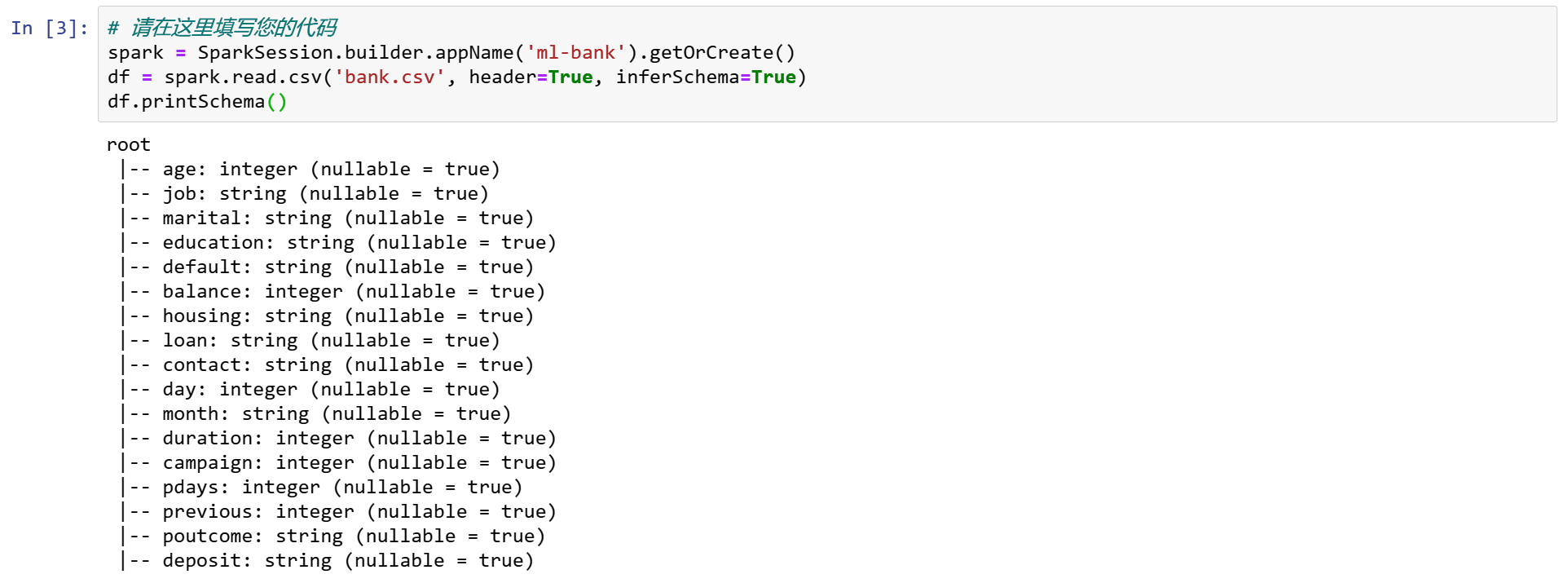
输入变量:
- age, job, marital, education, default, balance, housing, loan, contact, day, month, duration, campaign, pdays, previous, poutcome.
输出变量: - deposit
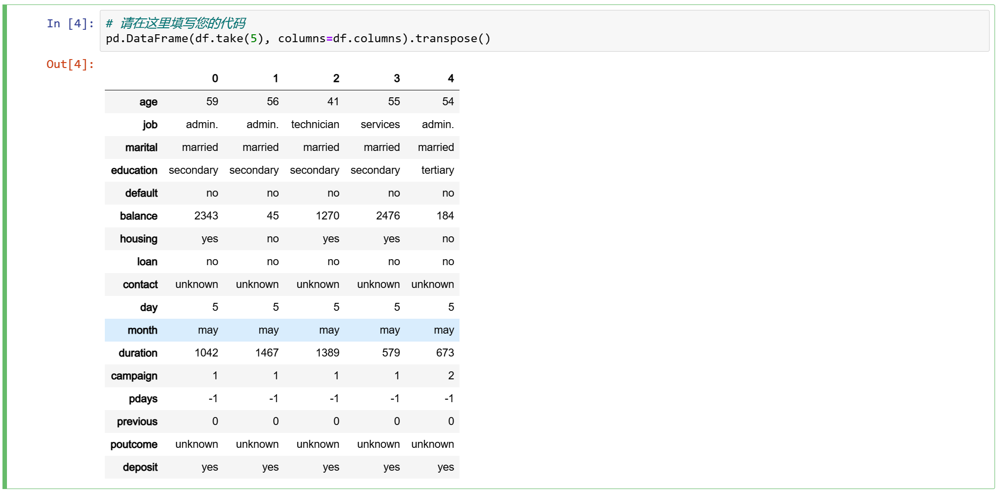
步骤3 查看前五个观测样本
3.1 pandas.DataFrame 比 Spark DataFrame.show()更漂亮
pd.DataFrame(df.take(5), columns=df.columns).transpose()
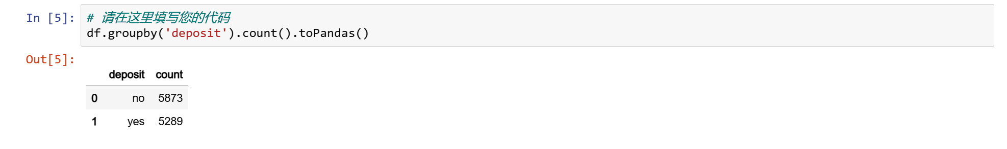
3.2 查看数据标签
df.groupby('deposit').count().toPandas()
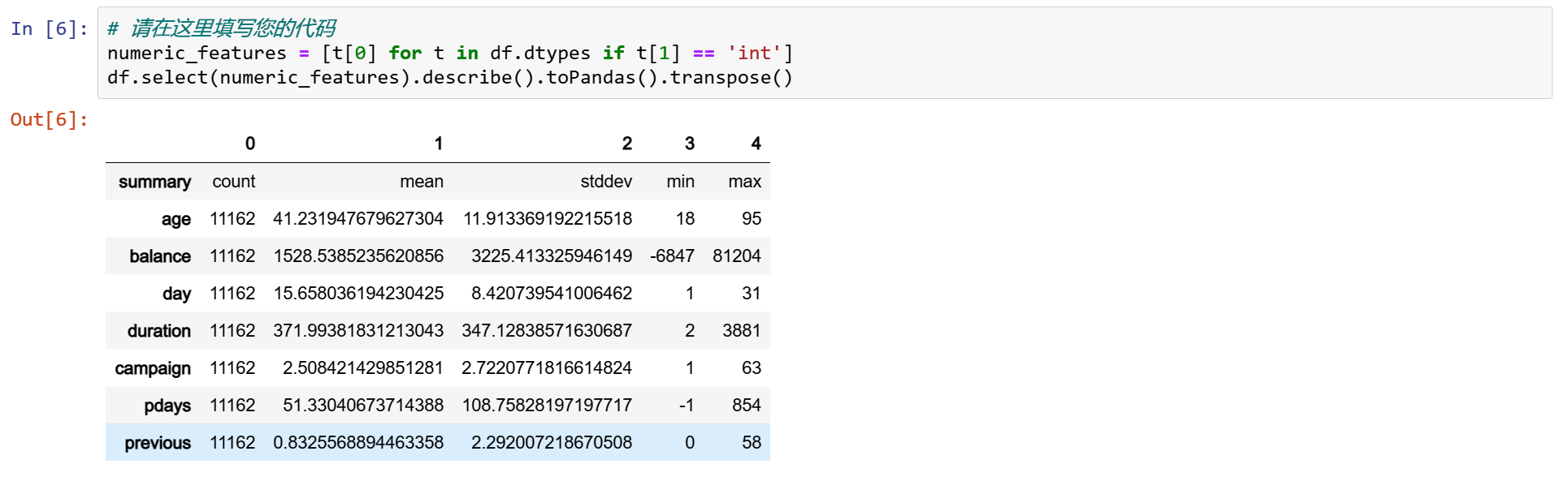
3.3 数值变量的汇总统计信息
numeric_features = [t[0] for t in df.dtypes if t[1] == 'int']
df.select(numeric_features).describe().toPandas().transpose()
3.4 变量的相关性检验
numeric_data = df.select(numeric_features).toPandas()

axs = pd.plotting.scatter_matrix(numeric_data, figsize=(8, 8));

# 旋转轴标签并移除轴刻度
n = len(numeric_data.columns)
for i in range(n):
    v = axs[i, 0]
    v.yaxis.label.set_rotation(0)
    v.yaxis.label.set_ha('right')
    v.set_yticks(())
    h = axs[n-1, i]
    h.xaxis.label.set_rotation(90)
    h.set_xticks(())
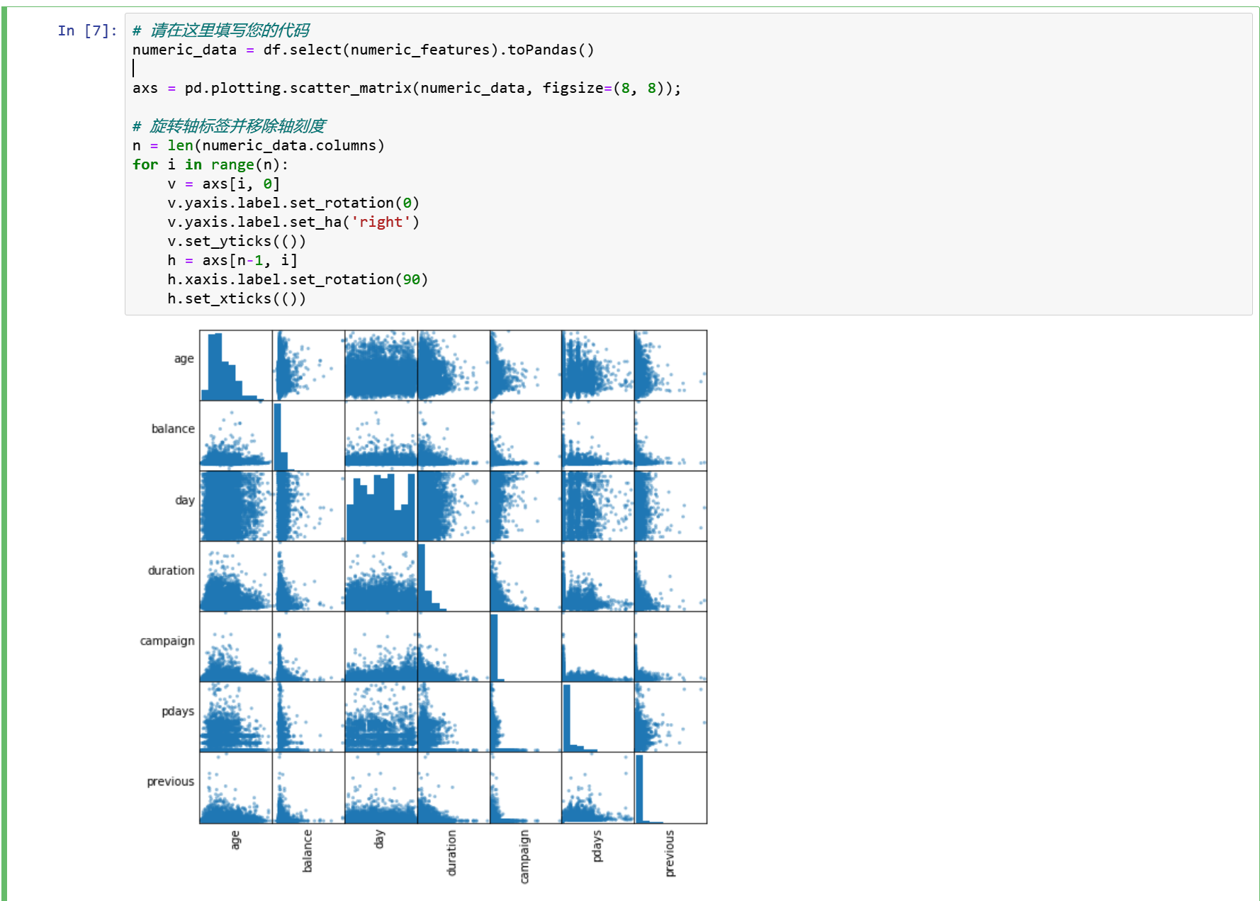
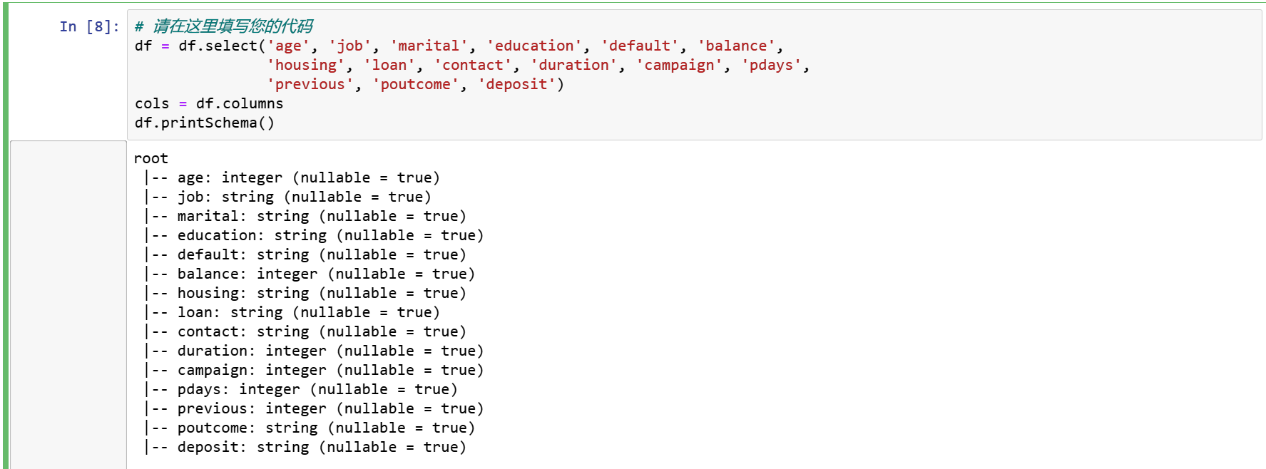
很明显,没有高度相关的自变量。因此,我们将保留所有的变量。然而,日列和月列并不是很有用,我们将删除这两列。
df = df.select('age', 'job', 'marital', 'education', 'default', 'balance',
               'housing', 'loan', 'contact', 'duration', 'campaign', 'pdays',
               'previous', 'poutcome', 'deposit')
cols = df.columns
df.printSchema()
3.5 为机器学习准备数据
分类索引,一个One-Hot和向量汇编器,一个特征转换器,合并多个列成一个向量列。
categoricalColumns = [
    'job', 'marital', 'education', 'default', 'housing', 'loan', 'contact',
    'poutcome'
]
stages = []

for categoricalCol in categoricalColumns:
    stringIndexer = StringIndexer(inputCol=categoricalCol,
                                  outputCol=categoricalCol + 'Index')
    encoder = OneHotEncoderEstimator(inputCols=[stringIndexer.getOutputCol()],
                                     outputCols=[categoricalCol + "classVec"])
    stages += [stringIndexer, encoder]

label_stringIdx = StringIndexer(inputCol='deposit', outputCol='label')
stages += [label_stringIdx]

numericCols = ['age', 'balance', 'duration', 'campaign', 'pdays', 'previous']
assemblerInputs = [c + "classVec" for c in categoricalColumns] + numericCols
assembler = VectorAssembler(inputCols=assemblerInputs, outputCol="features")
stages += [assembler]
上面的代码取自 databricks 的官方站点,它使用 StringIndexer 对每个分类列进行索引,然后将索引的类别转换为一个one-hot变量。
得到的输出将二进制向量附加到每一行的末尾。
我们再次使用 StringIndexer 将标签编码为标签索引。
接下来,我们使用 VectorAssembler 将所有特性列组合成一个向量列。
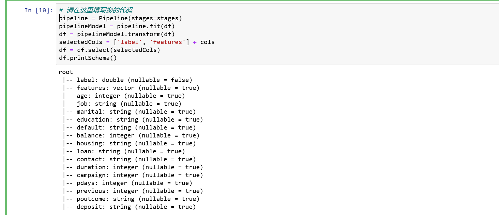
3.6 管道
我们使用管道将多个转换器和评估器链接在一起,以指定我们的机器学习工作流。管道的阶段被指定为有序数组。
pipeline = Pipeline(stages=stages)
pipelineModel = pipeline.fit(df)
df = pipelineModel.transform(df)
selectedCols = ['label', 'features'] + cols
df = df.select(selectedCols)
df.printSchema()
pd.DataFrame(df.take(5), columns=df.columns).transpose()
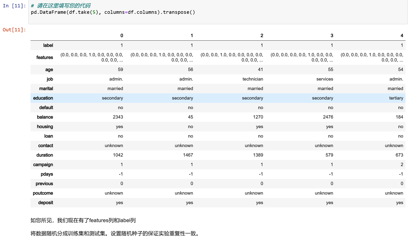
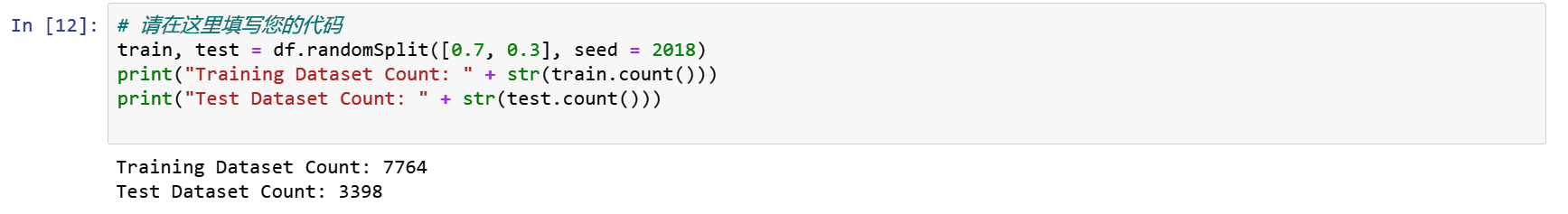
将数据随机分成训练集和测试集。设置随机种子的保证实验重复性一致。
train, test = df.randomSplit([0.7, 0.3], seed = 2018)
print("Training Dataset Count: " + str(train.count()))
print("Test Dataset Count: " + str(test.count()))
步骤4 逻辑回归
lr = LogisticRegression(featuresCol='features', labelCol='label', maxIter=10)
lrModel = lr.fit(train)
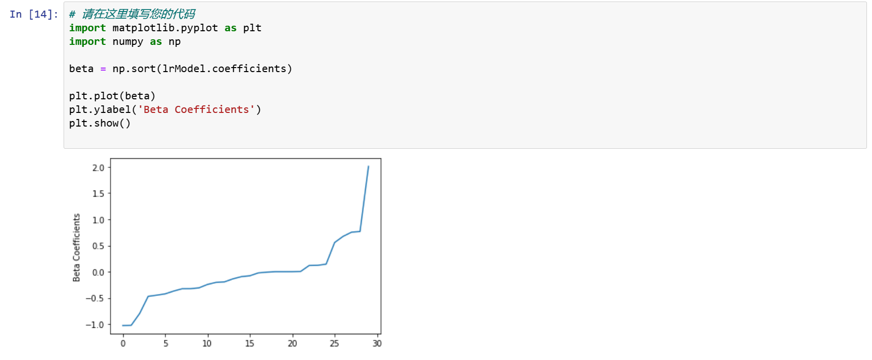
我们可以利用逻辑回归模型的属性得到回归系数与回归参数。
import matplotlib.pyplot as plt
import numpy as np

beta = np.sort(lrModel.coefficients)

plt.plot(beta)
plt.ylabel('Beta Coefficients')
plt.show()
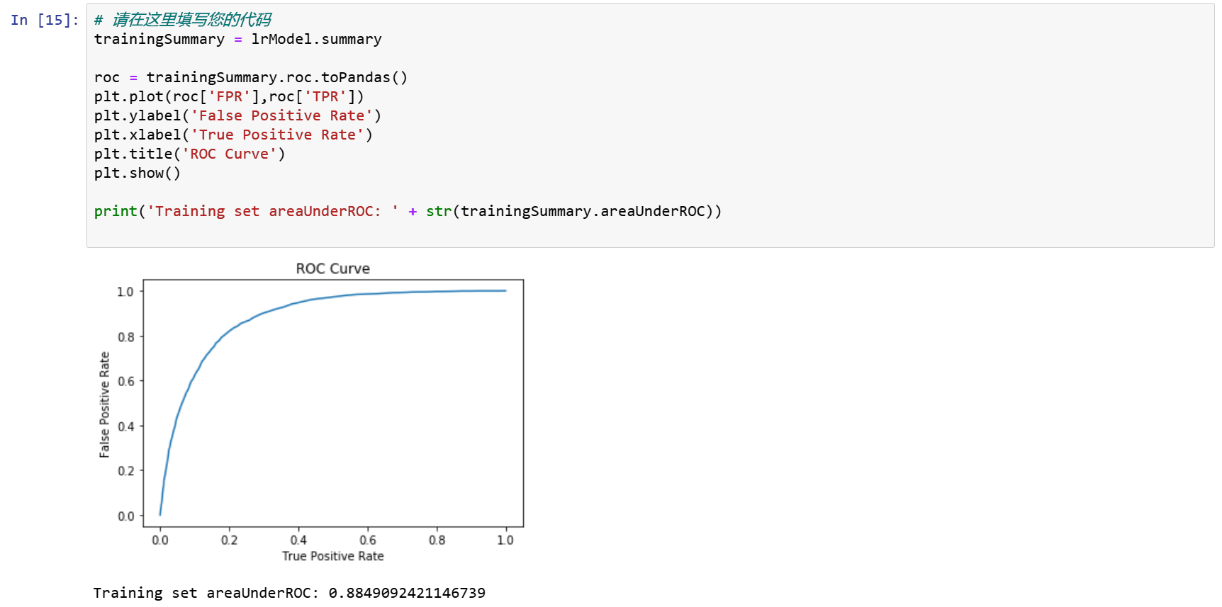
trainingSummary = lrModel.summary

roc = trainingSummary.roc.toPandas()
plt.plot(roc['FPR'],roc['TPR'])
plt.ylabel('False Positive Rate')
plt.xlabel('True Positive Rate')
plt.title('ROC Curve')
plt.show()

print('Training set areaUnderROC: ' + str(trainingSummary.areaUnderROC))
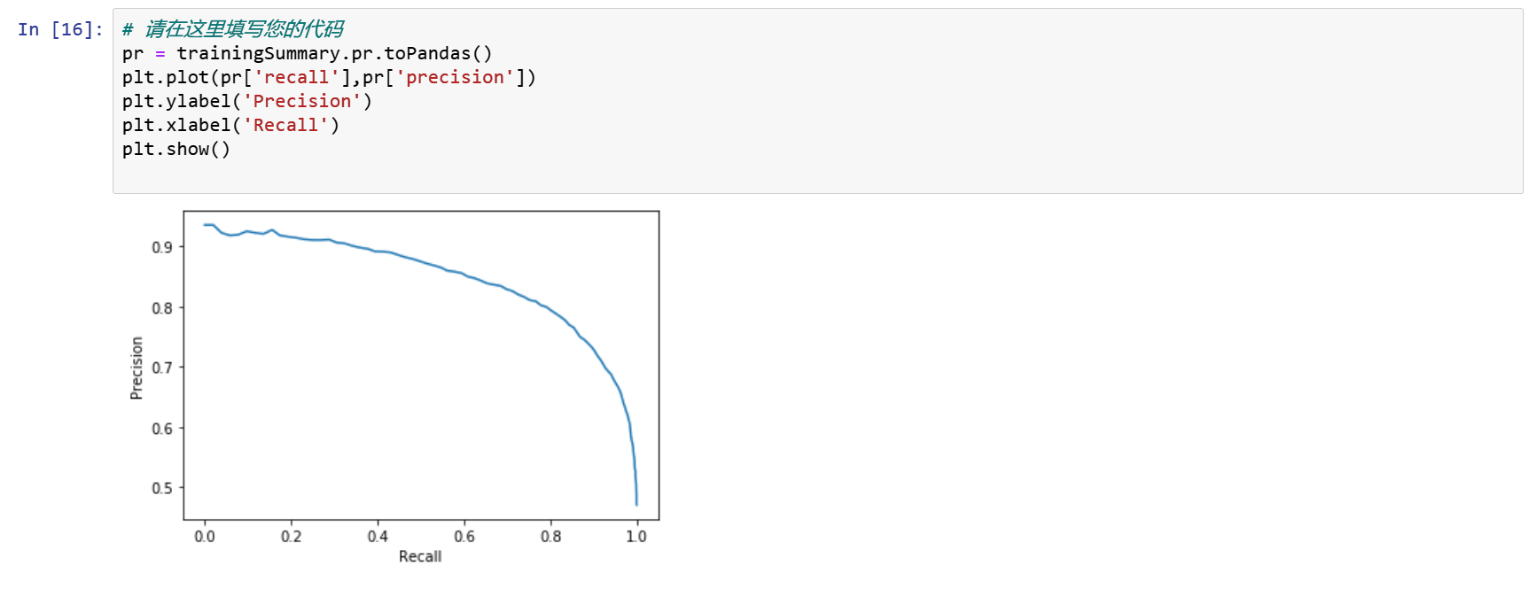
精度和召回 Precision and Recall
pr = trainingSummary.pr.toPandas()
plt.plot(pr['recall'],pr['precision'])
plt.ylabel('Precision')
plt.xlabel('Recall')
plt.show()
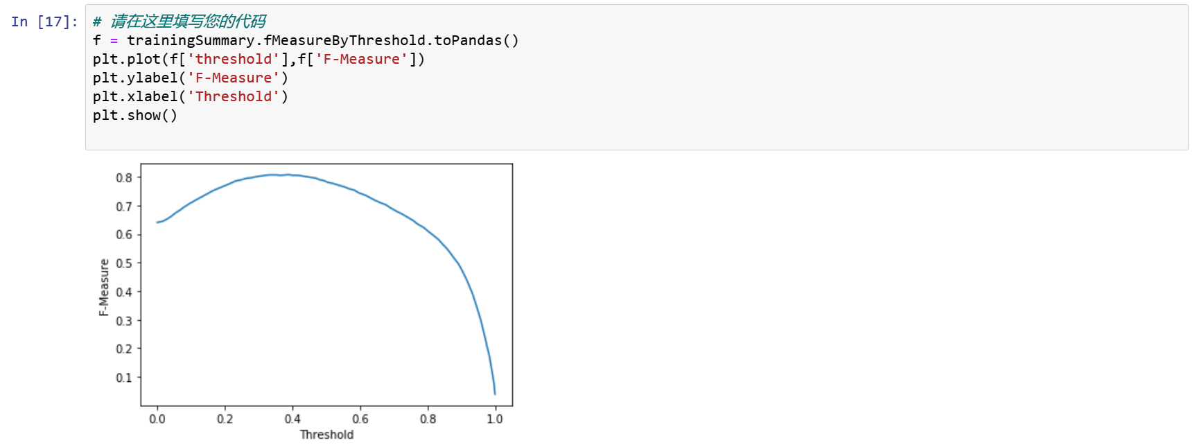
设置模型阈值,使F-Measure最大化
f = trainingSummary.fMeasureByThreshold.toPandas()
plt.plot(f['threshold'],f['F-Measure'])
plt.ylabel('F-Measure')
plt.xlabel('Threshold')
plt.show()
对测试集进行预测
predictions = lrModel.transform(test)
predictions.select('age', 'job', 'label', 'rawPrediction', 'prediction', 'probability').show(10)

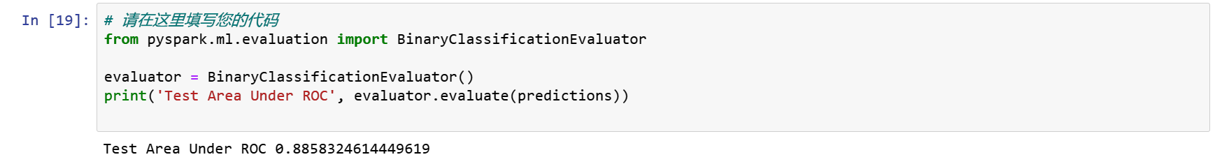
评估我们的逻辑回归模型
from pyspark.ml.evaluation import BinaryClassificationEvaluator

evaluator = BinaryClassificationEvaluator()
print('Test Area Under ROC', evaluator.evaluate(predictions))
evaluator.getMetricName()

模型训练的很好。
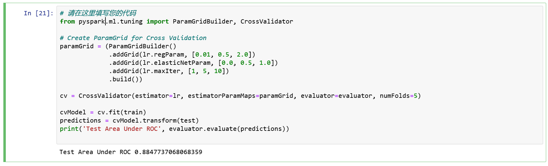
尝试使用ParamGridBuilder和CrossValidator对模型进行调优。
from pyspark.ml.tuning import ParamGridBuilder, CrossValidator

# Create ParamGrid for Cross Validation
paramGrid = (ParamGridBuilder()
             .addGrid(lr.regParam, [0.01, 0.5, 2.0])
             .addGrid(lr.elasticNetParam, [0.0, 0.5, 1.0])
             .addGrid(lr.maxIter, [1, 5, 10])
             .build())

cv = CrossValidator(estimator=lr, estimatorParamMaps=paramGrid, evaluator=evaluator, numFolds=5)

cvModel = cv.fit(train)
predictions = cvModel.transform(test)
print('Test Area Under ROC', evaluator.evaluate(predictions))
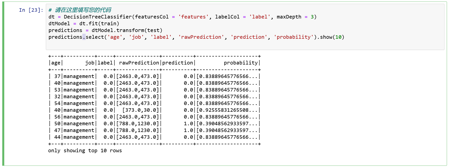
步骤5 决策树分类器
决策树由于易于解释、处理分类特征、扩展到多类分类设置、不需要特征缩放以及能够捕获非线性和特征交互而被广泛使用。
dt = DecisionTreeClassifier(featuresCol = 'features', labelCol = 'label', maxDepth = 3)
dtModel = dt.fit(train)
predictions = dtModel.transform(test)
predictions.select('age', 'job', 'label', 'rawPrediction', 'prediction', 'probability').show(10)
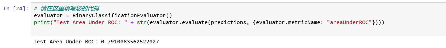
评估我们的决策树模型
evaluator = BinaryClassificationEvaluator()
print("Test Area Under ROC: " + str(evaluator.evaluate(predictions, {evaluator.metricName: "areaUnderROC"})))
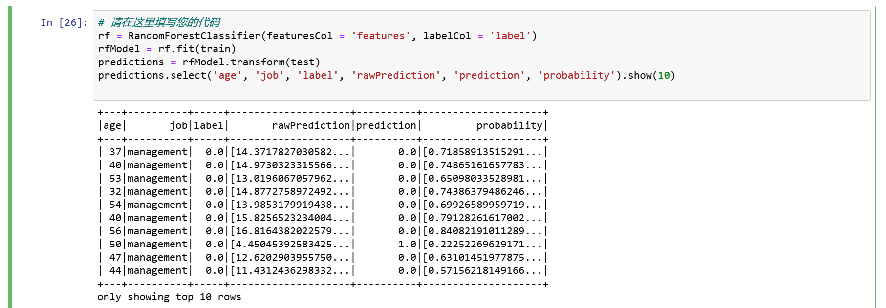
步骤6 随机森林分类器
rf = RandomForestClassifier(featuresCol = 'features', labelCol = 'label')
rfModel = rf.fit(train)
predictions = rfModel.transform(test)
predictions.select('age', 'job', 'label', 'rawPrediction', 'prediction', 'probability').show(10)
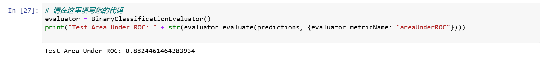
evaluator = BinaryClassificationEvaluator()
print("Test Area Under ROC: " + str(evaluator.evaluate(predictions, {evaluator.metricName: "areaUnderROC"})))
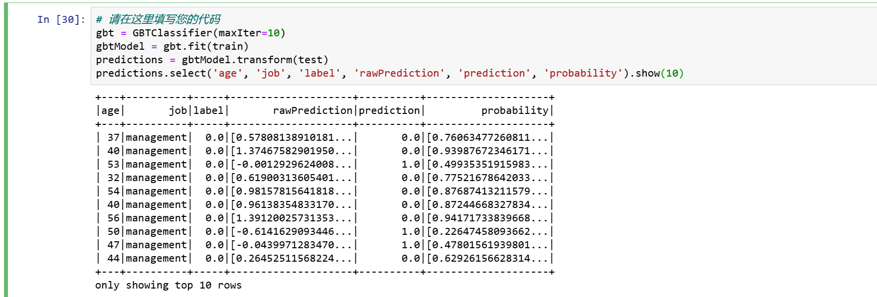
步骤7 Gradient-boosted树分类器
gbt = GBTClassifier(maxIter=10)
gbtModel = gbt.fit(train)
predictions = gbtModel.transform(test)
predictions.select('age', 'job', 'label', 'rawPrediction', 'prediction', 'probability').show(10)
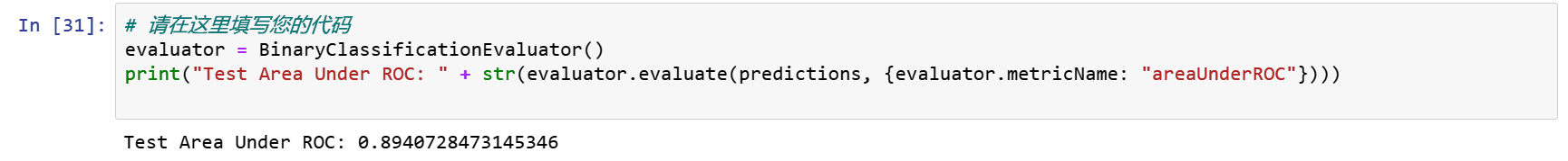
evaluator = BinaryClassificationEvaluator()
print("Test Area Under ROC: " + str(evaluator.evaluate(predictions, {evaluator.metricName: "areaUnderROC"})))
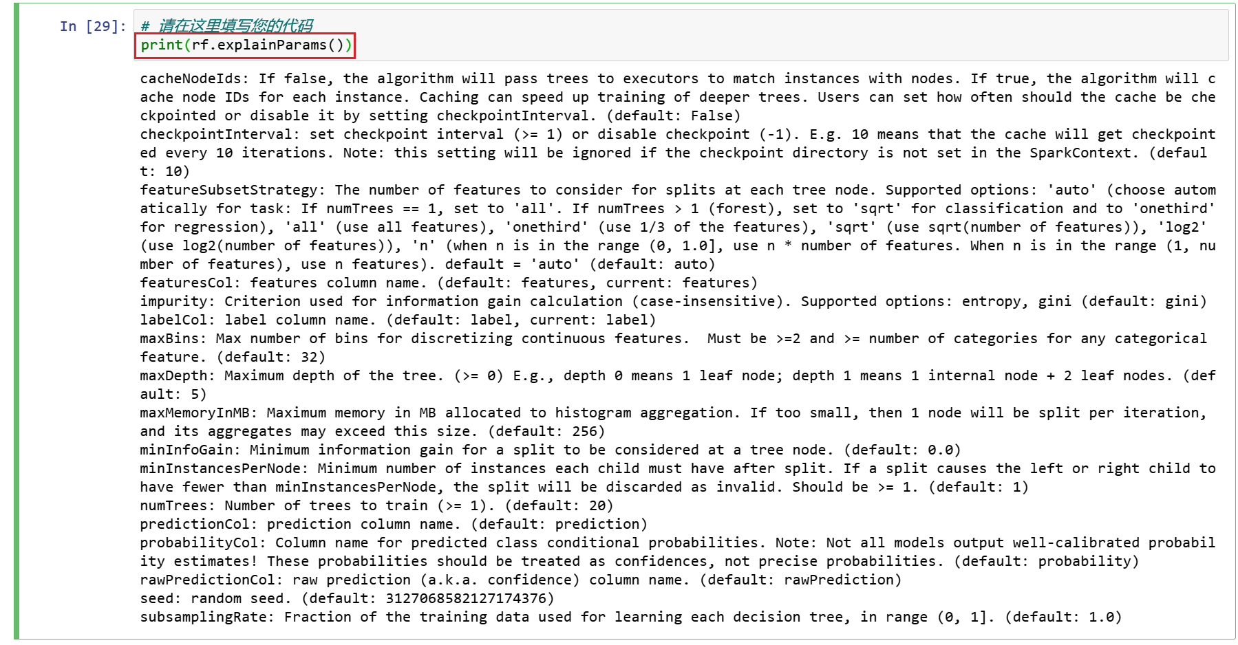
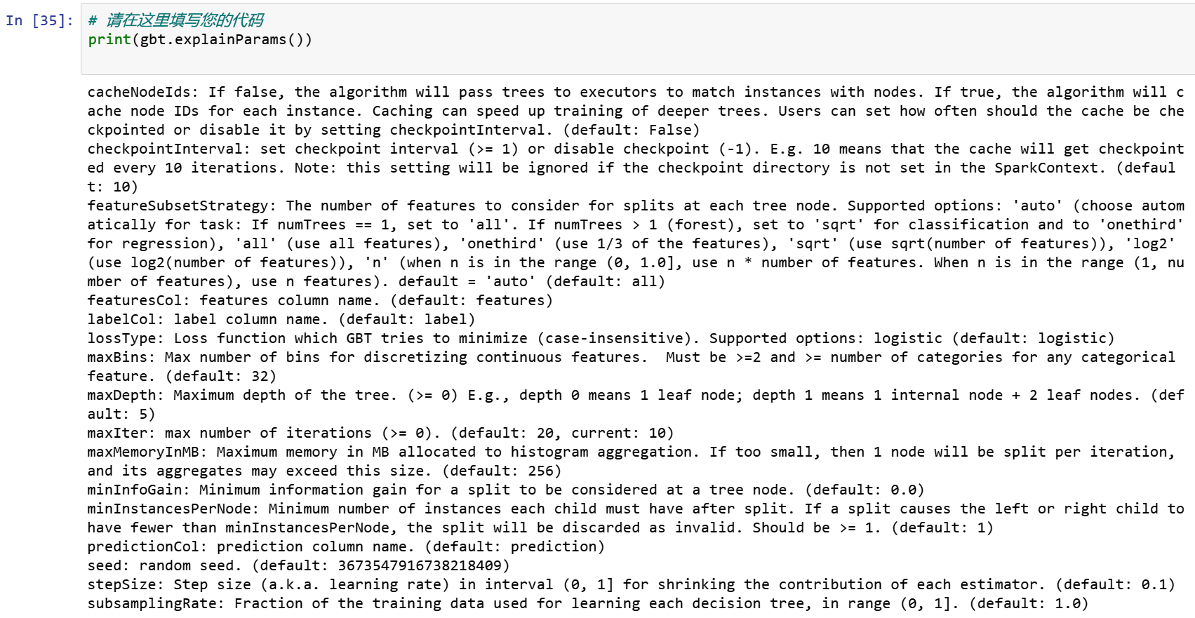
Gradient-boosted树获得了最好的结果,我们将尝试使用ParamGridBuilder和CrossValidator对这个模型进行调优。
在此之前,我们可以使用explainParams()打印所有params及其定义的列表,以了解哪些params可用于调优。
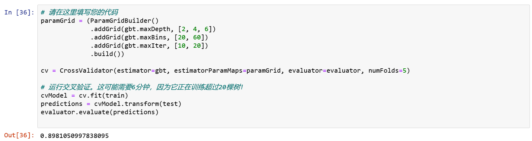
paramGrid = (ParamGridBuilder()
             .addGrid(gbt.maxDepth, [2, 4, 6])
             .addGrid(gbt.maxBins, [20, 60])
             .addGrid(gbt.maxIter, [10, 20])
             .build())

cv = CrossValidator(estimator=gbt, estimatorParamMaps=paramGrid, evaluator=evaluator, numFolds=5)

# 运行交叉验证。这可能需要6分钟,因为它正在训练超过20棵树!
cvModel = cv.fit(train)
predictions = cvModel.transform(test)
evaluator.evaluate(predictions)
总之,我们学习了如何使用PySpark和MLlib pipeline API构建一个二进制分类应用程序。
我们尝试了四种算法,Gradient Boosting在我们的数据集中表现得最好。
思考
随机森林和Gradient Boosting都属于集成学习的算法,为什么在准确率和ROC上,后者明显好于前者?
GBM采用boosting技术做预测。在bagging技术中,数据集用随机采样的方法被划分成使n个样本。然后,使用单一的学习算法,在所有样本上建模。接着利用投票或者求平均来组合所得到的预测。
Bagging是平行进行的。而boosting是在第一轮的预测之后,算法将分类出错的预测加高权重,使得它们可以在后续一轮中得到校正。这种给予分类出错的预测高权重的顺序过程持续进行,一直到达到停止标准为止。随机森林通过减少方差(主要方式)提高模型的精度。生成树之间是不相关的,以把方差的减少最大化。在另一方面,GBM提高了精度,同时减少了模型的偏差和方差。


 8648
8648


 被折叠的 条评论
为什么被折叠?
被折叠的 条评论
为什么被折叠?
 到【灌水乐园】发言


