


翻译自:Polyline Simplification - CodeProject
参考:Polyline Simplification - CodeProject
整个记录关于算法的部分是翻译来的,原作者实现的语言是C++,但是我看不懂这类代码,于是自己用Python实现了一遍,其中可能会有错误的地方,欢迎指出来让我改正。
标注原创的原因是翻译未获得作者授权(联系不上),要是以后联系上再改吧。
In [1]:
from shapefile import Reader, Writer
import numpy as np
import math
import matplotlib.pyplot as plt
In [26]:
# 该shapefile文件内含一条线段,坐标系为:3857
shp = Reader('./vector/lyr_line.shp', encoding='utf-8')
In [3]:
feat = shp.shape(0)
line = np.array(feat.points)
In [4]:
# 保存为shapefile文件
def shpGen(fileName, pts):
    w = Writer(fileName, encoding='utf-8', shapeType=3)
    w.fields = shp.fields
    w.line([pts])
    w.record("测试", 3)
    w.close()
In [5]:
# 点到线距离
def point2lineDistance(x0,y0,x1,y1,x2,y2):
    a =x2 -x1
    b = y2 - y1
    c = b*x1-  a*y1
    return abs(a*y0 - b*x0 + c) / math.sqrt(a*a + b*b)
    # return abs((x2-x1)*(y1-y0)-(x1-x0)*(y2-y1)) / math.sqrt((x2-x1)*(x2-x1)+(y2-y1)*(y2-y1))
# 点到点距离
def point2pointDistance(x1,y1,x2,y2):
    dx = x2-x1
    dy = y2-y1
    return math.sqrt(dx*dx+dy*dy)

# 绘制
def plotLine(pts, simplifyLst, newlabel:str):
    plt.figure(figsize=(15, 6))
    plt.plot(pts[:,0], pts[:,1], 'r-*', linewidth=0.5, mfc='red', mec='red', label='origin')
    plt.plot(simplifyLst[:,0], simplifyLst[:,1], 'b-s', linewidth=0.5, mfc='blue', mec='blue', label=newlabel)
    plt.legend(loc='upper left')
    plt.show()
Radial Distance
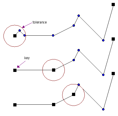
该算法是一个时间复杂度为${O(n)}$的暴力算法。在连续的顶点中,与当前某一个key(简化过程中标记保留的顶点)的距离太近时会被去掉。
起止顶点一般会保留作为简化线的一部分,故标记为key,从第一个key(第一个顶点)开始,算法将遍历整条线段,所有连续顶点中,移除那些距离不超过容忍值的顶点,而第一个超过容忍值的顶点将标记为下一个key,从新key开始,算法重新遍历余下的点并重复上述过程,直到最后一个点。
In [6]:
def NearestSimplify(tolorence:float, pts:list) -> list:
    start = 0
    validFlags = np.zeros((len(pts), ), dtype="bool")
    for i in range(1, len(pts)):
        dist = math.sqrt(math.pow(pts[i][0]- pts[start][0], 2) +
                         math.pow(pts[i][1] - pts[start][1], 2))
        if dist > tolorence:
            validFlags[i] = True
            start = i
    validFlags[0] = True
    return validFlags
In [7]:
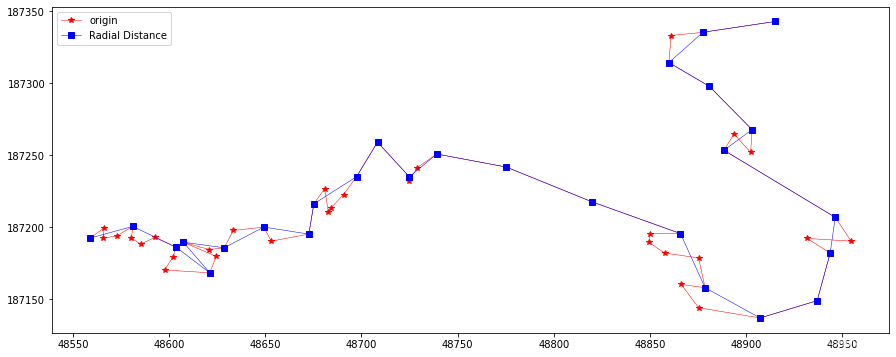
flags =  NearestSimplify(20, feat.points)
plotLine(line, line[flags], "Radial Distance")
In [8]:
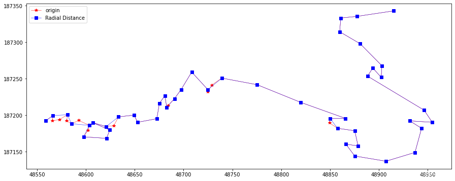
flags =  NearestSimplify(10, feat.points)
plotLine(line, line[flags], "Radial Distance")
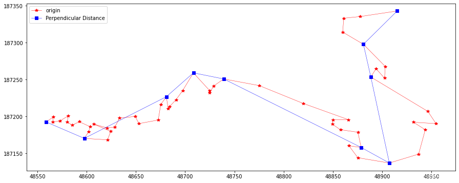
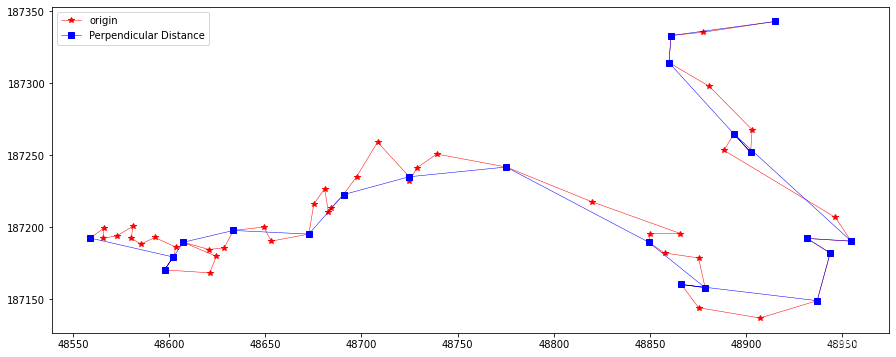
Perpendicular Distance
临近点算法将点-点距离作为误差判据,而垂直距离简化则是将点-线段的距离作为误差判据。对于每个顶点Vi,需要计算它与线段[Vi-1, Vi+1]的垂直距离,距离小于给定容忍值的点将被移除。过程如下图所示:

正在上传…重新上传取消
最开始处理前三个顶点,计算第二个顶点的垂直距离,与容忍值作比较,大于则标记为key。然后算法往前移动开始处理下一个前三个顶点,第二次距离小于容忍值,移除中间顶点。重复直到处理所有顶点。
注意:对于每个被移除的顶点Vi,下一个可能被移除的候选顶点是Vi+2。这意味着原始多段线的点数最多只能减少50%。为了获得更高的顶点减少率,需要多次遍历。
In [27]:
def PerpendicularSimplify(tolorence:float, pts:list) -> list:
    sp = 0
    ep = 2
    validFlags = np.zeros((len(pts), ), dtype="bool")
    for i in range(1, len(pts) - 1):
        verDist = point2lineDistance(
            pts[i][0], pts[i][1],
            pts[sp][0], pts[sp][1],
            pts[ep][0], pts[ep][1])
        if verDist > tolorence:
            validFlags[i] = True
            sp = i
            ep = i + 2
    validFlags[0] = validFlags[-1] = True
    return validFlags
In [10]:
perLine = PerpendicularSimplify(20, feat.points)
plotLine(line, line[perLine], "Perpendicular Distance")
In [11]:
perLine = PerpendicularSimplify(10, feat.points)
plotLine(line, line[perLine], "Perpendicular Distance")
Reumann-Witkam
该算法使用点-线距离作距离判断。首先定义一条线段,起止点为原始线段的前两个顶点,对于每一个连续的顶点vi,计算它与前述线段的垂直距离,当距离超过容忍值时,将顶点vi - 1标记为key。顶点vi和vi + 1用来定义新的线段,算法重复直到最后一个点。下图为算法演示:
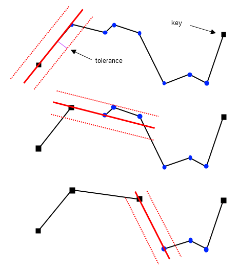
红色的条带由指定的容忍值生成,而线段则由原始线的前两个顶点生成。第三个顶点不在红色条带内,意味着该顶点是一个key。通过第二,三顶点定义新的条带,位于条带内的最后一个顶点也标记为key,而其他点则移除。算法重复直到新吊带包含原始线段的最后一个顶点。
In [12]:
def ReuWitkamSimplify(tolorence:float, pts:list) -> list:
    sp = 0
    ep = 1
    validFlags = np.zeros((len(pts), ), dtype="bool")
    for i in range(2, len(pts)):
        verDist = point2lineDistance(
            pts[i][0], pts[i][1],
            pts[sp][0], pts[sp][1],
            pts[ep][0], pts[ep][1])
        if verDist > tolorence:
            validFlags[i-1] = True
            sp = ep
            ep = i
    validFlags[0] = validFlags[-1] = True
    return validFlags
In [13]:
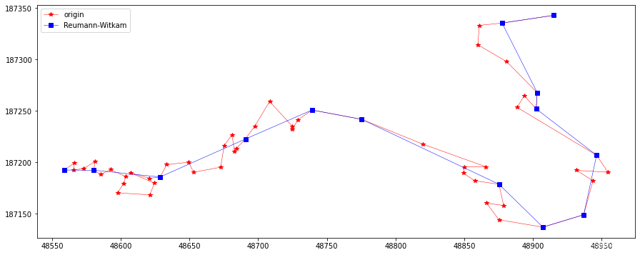
rLine = ReuWitkamSimplify(20, feat.points)
plotLine(line, line[rLine], "Reumann-Witkam")
In [14]:
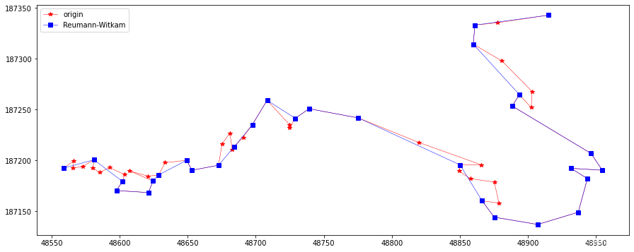
rLine = ReuWitkamSimplify(10, feat.points)
plotLine(line, line[rLine], "Reumann-Witkam")
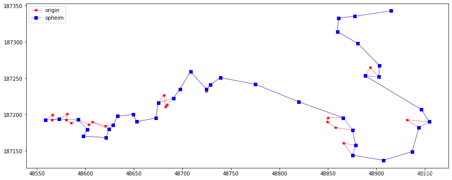
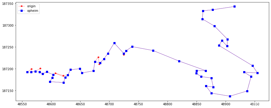
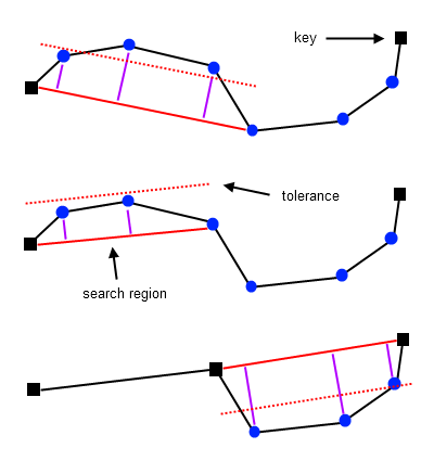
Opheim
Ophein 使用 最小和最大距离容忍值来约束搜索区域。对于连续的顶点vi,它与当前key(通常是v0的径向距离可以被计算出来。在容忍值范围内的最后一个顶点被用来定义一条射线R(vkey, vi),如果这样的顶点不存在,那么射线将被定义为R(vkey, vkey + 1)。计算每一个连续的顶点vj(在vi后边)与射线R间的垂直距离, 当该距离超过最小容忍值或者当vj与vkey间的辐射距离大于最大容忍值时,在vj-1位置上的顶点,将被认为是一个新key。

正在上传…重新上传取消
值得注意的是,关于如何定义射线${R(v_{key},v_i)}$ 去控制搜索区域的方法存在多个,可能的方法有如下几种:
- Reumann-Witkam 的方法 : ${i}$ = ${key}$ + 1.
- 外部第一个点:${key}$ < ${i}$ 且${v_i}$ 是第一个掉落在最小辐射距离外部的点.
- 内部最后一个点:${key}$ < ${i}$ 且 ${v_i}$ 是掉落在最小辐射距离内的最后一个点;若该点不存在,则使用方法1.

正在上传…重新上传取消
In [31]:
def opheimSimplify(minTolorence:int, maxTolorence:int, pts) -> list:
    vKey = 0
    validPtsLst = np.zeros((len(pts),), dtype='bool')
    for i in range(vKey, len(pts)):
        if point2pointDistance(pts[vKey][0], pts[vKey][1], pts[i][0], pts[i][1]) > minTolorence:
            vi = i
            break
    for j in range(vi + 1, len(pts)):
        vj2rayDist = point2lineDistance(
            pts[j][0], pts[j][1],
            pts[vKey][0], pts[vKey][1],
            pts[vi][0], pts[vi][1])
        radialDist = point2pointDistance(pts[vKey][0], pts[vKey][1], pts[j][0], pts[j][1])
        if vj2rayDist <= minTolorence or radialDist > maxTolorence:
            vKey = j - 1
            validPtsLst[j-1] = True
        else:
            continue
    validPtsLst[0] = validPtsLst[-1]= True
    return np.array(validPtsLst)
In [16]:
opheim = opheimSimplify(2, 20, np.array(feat.points))
plotLine(line, line[opheim], "opheim")
In [17]:
opheim = opheimSimplify(2, 10, np.array(feat.points))
plotLine(line, line[opheim], "opheim")
Lang
Lang 简化算法定义一个固定大小的搜索区域,它的第一个和最后一个点来自线段的同一个片段——用来计算处于中间的顶点的垂直距离。若任何计算出的距离大于指定的容忍值,那么搜索区域将通过排除其最后一个顶点进行收缩,这个过程会一直重复直到所有垂直距离小于特定的容忍值,或者中间顶点全部排除。所有中间节点移除后,新的搜索区域将以旧搜索区域的最后一个点作为起点进行构建。
搜索区域使用前四个顶点来生成。计算每一个中间顶点到片段S(v0, v4)的垂直距离,只要至少存在一个顶点的垂直距离超过容忍值,搜索区域便简化一个顶点。再重复计算中间顶点到片段S(v0, v3),所有的中间顶点到片段S的垂直距离都位于容忍值内,搜索区域的最后一个顶点v3作为一个新key同时它也用来定义一个新的区域(片段)S(v3, v7)。
- 第一个点作为vKey,创建片段S(v0, v4)
- 求中间顶点到片段的垂直距离
- 片段依次排除最后一个顶点(当距离超过容忍值)
- 片段内无顶点的垂直距离超过容忍值,此时最后一个点作为新key,同时构建新片段
- 重复1-4
In [18]:
def langSimplify(tolorence, pts, steps=0) -> list:
    vKey = 0
    end = 2
    validLst = np.zeros((len(pts),), dtype='bool')
    if(steps == 0):
        maxSteps = len(pts) - 1
    else:
        maxSteps = steps
    while  vKey < maxSteps and end < maxSteps:
        isBigger = False
        # print("segment:(%s,%s)" % (vKey, end))
        for i in range(vKey + 1, end):
            perDist = point2lineDistance(
                pts[i][0], pts[i][1],
                pts[vKey][0], pts[vKey][1],
                pts[end][0], pts[end][1])
            if perDist > tolorence:
                isBigger = True
                end -= 1
                break
            else:
                continue
        if not isBigger:
            vKey = end
            end += 2
            validLst[vKey] = True
    validLst[0] = validLst[-1] = True
    return validLst
In [19]:
langLine = langSimplify(20, feat.points, steps=0)
plotLine(line, line[langLine], "Lang")

In [20]:
langLine = langSimplify(10, feat.points, steps=0)
plotLine(line, line[langLine], "Lang")

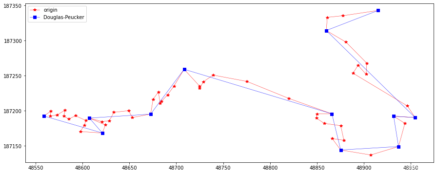
Douglas-Peucker
Douglas-Peucker算法使用点-边距离作为误差衡量标准。该算法从连接原始Polyline的第一个和最后一个顶点的边开始,计算所有中间顶点到边的距离,距离该边最远的顶点,如果其距离大于指定的公差,将被标记为Key并添加到简化结果中。这个过程将对当前简化中的每条边进行递归,直到原始Polyline的所有顶点与当前考察的边的距离都在允许误差范围内。该过程如下图所示:
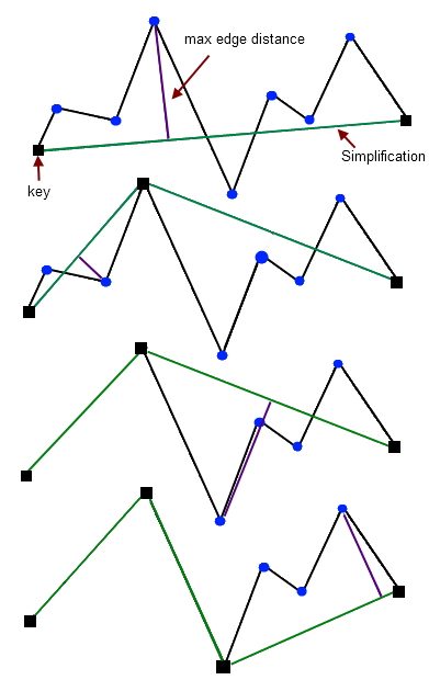
初始时,简化结果只有一条边(起点-终点)。第一步中,将第四个顶点标记为一个Key,并相应地加入到简化结果中;第二步,处理当前结果中的第一条边,到该边的最大顶点距离低于容差,因此不添加任何点;在第三步中,当前简化的第二个边找到了一个Key(点到边的距离大于容差)。这条边在这个Key处被分割,这个新的Key添加到简化结果中。这个过程一直继续下去,直到找不到新的Key为止。注意,在每个步骤中,只处理当前简化结果的一条边。
In [22]:
def douglasPeuckerSimplify(tolorence, pts) -> list:
    start = 0
    end = len(pts) - 1
    def findPt(start, end):
        curPt = 0
        maxDist = 0
        for i in range(start + 1, end):
            perpenDist = point2lineDistance(
                pts[i][0], pts[i][1],
                pts[start][0], pts[start][1],
                pts[end][0], pts[end][1])
            if perpenDist > maxDist:
                maxDist = perpenDist
                curPt = i
        if maxDist > tolorence:
            preKey = findPt(start, curPt)
            postKey = findPt(curPt, end)
            return [] + preKey + postKey
        else:
            return [pts[end]]
    return [pts[0]] + findPt(start, end)
In [23]:
res = douglasPeuckerSimplify(20, feat.points)
plotLine(line, np.array(res), "Douglas-Peucker")
In [24]:
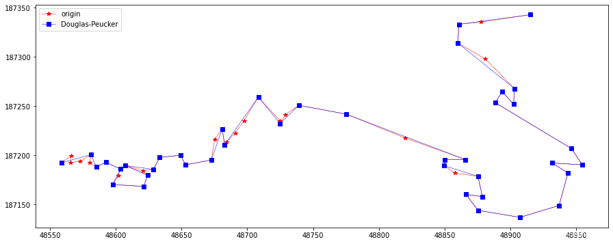
res = douglasPeuckerSimplify(10, feat.points)
plotLine(line, np.array(res), "Douglas-Peucker")

In [25]:
res = douglasPeuckerSimplify(5, feat.points)
plotLine(line, np.array(res), "Douglas-Peucker")
In [ ]:


 16万+
16万+


 被折叠的 条评论
为什么被折叠?
被折叠的 条评论
为什么被折叠?
 到【灌水乐园】发言


