线性回归、逻辑回归

实验二、三：线性回归、逻辑回归

实验内容：掌握线性回归和逻辑回归的方法

实验过程：

1.实验思想：

1.1线性回归: 监督学习算法

1.1.1单变量线性回归：

只含有一个特征/输入变量，因此这样的问题叫作单变量线性回归问题，表达方式为： 。代价函数定义（误差平方和代价函数）:  ，通过计算使代价函数最小，从而确定系数即可，采用梯度下降的方法来实现，具体的算法如下：

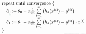
注意有可能出现假最优值的点。

1.1.2多变量线性回归：

       多变量线性回归主要是多了特征/输入变量，下面给出梯度下降算法的公式：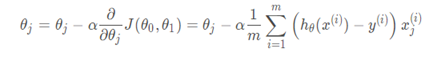

 进行归一化处理

2.1逻辑回归

Logistic Regression 为回归，但其实际上是分类模型，并常用于二分类

2.    源代码

2.1.1

import numpy as np

import matplotlib.pyplot as plt

a = np.loadtxt('./ex1data1.txt')

m=a.shape[0]

print(m)

print(type(a))

x=a[:,0]

y=a[:,1]

plt.scatter(x,y,marker='*',color='r',s=20)

theta0=0

theta1=0

iterations = 1500

alpha = 0.01

def gradientdescent(x,y,theta0,theta1,iterations,alpha):

    J_h=np.zeros( (iterations,1) )

    for i in range(0,iterations):

        y_hat=theta0+theta1*x

        temp0=theta0-alpha*((1/m)*sum(y_hat-y))

        temp1=theta1-alpha*(1/m)*sum((y_hat-y)*x)

        theta0=temp0

        theta1=temp1

        y_hat2=theta0+theta1*x

        aa=sum((y_hat2-y)**2)

        J=aa*(1/(2*m))

        J_h[i,:]=J

    return theta0,theta1,J_h



(theta0,theta1,J_h) = gradientdescent(x,y,theta0,theta1,iterations,alpha)

print(theta1)

print(theta0)

plt.plot(x,theta0+theta1*x)

plt.title("fittingcurve")

plt.show()

x2=np.arange(iterations)

plt.plot(x2,J_h)

plt.title("costfunction")

plt.show()

2.1.2

import numpy as np

import pandas as pd

import matplotlib

import matplotlib.pyplot as plt



matplotlib.rcParams['font.sans-serif']=['SimHei']



path="./ex1data2.txt"

data=pd.read_csv(path, header=None, names=['size','num','price'])

data.head()

X= data.loc[:, ['size', 'num']]

y= data.loc[:, 'price']

X= (X - X.mean()) / X.std()

X.insert(0, 'ones', 1)

X.head()





X=np.matrix(X.values)

y=np.matrix(y.values)

theta=(np.matrix([0,0,0])).T





def computeCost(x,y,theta):

    inner=np.sum(np.power((theta.T*x.T-y),2))

    return inner/(2*len(x))





def gradientDescent(x,y,theta,alpha,iters):

    temp=np.matrix(np.zeros(theta.shape))

    cost=np.zeros(iters)

    for i in range(iters):

        temp=theta-(alpha/len(x))*((theta.T*x.T-y)*x).T

        theta=temp

        cost[i]=computeCost(x,y,theta)

    return theta,cost





alpha=[0.0001,0.001,0.01,0.0003,0.003,0.03]

iters=2000



x=np.arange(iters)

fig,ax=plt.subplots()

for i in alpha:

    finally_theta,cost = gradientDescent(X, y, theta, i, iters)

    ax.plot(np.arange(iters), cost, label=i)

    ax.legend()

ax.set(xlabel='迭代次数',ylabel='代价函数值',title='代价函数曲线')

plt.show()

2.2

import numpy as np

import pandas as pd

import matplotlib.pyplot as plt

import scipy.optimize as opt #优化算法

from sklearn.metrics import classification_report

from sklearn import linear_model

# 获取原始数据

def raw_data(path):

    data=pd.read_csv(path,names=['exam1','exam2','admit'])

    return data

#绘制初始数据

#需要将两种判断结果区别颜色绘制

def draw_data(data):

    accept = data[data.admit==1]

    refuse = data[data.admit == 0]

    #accept=data[data['admit'].isin([1])]

    #refuse=data[data['admit'].isin([0])]

    plt.scatter(accept.exam1,accept.exam2,c='g',label = 'admit')

    plt.scatter(refuse.exam1,refuse.exam2,c='r',label = 'not admit')

    plt.title('admission')

    plt.xlabel('score1')

    plt.ylabel('score2')

    return plt

#sigmoid函数

def sigmoid(z):

    return 1/(1+np.exp(-z))#exp（-z）:e的-z次方

#代价函数

def cost_function(theta, x, y):

    m = x.shape[0]

    j = (y.dot(np.log(sigmoid(x.dot(theta))))+(1-y).dot(np.log(1-sigmoid(x.dot(theta)))))/(-m)

    return j

#计算偏导数即可，后面会用scipy.optimize中方法求最优解

def gradient_descent(theta, x, y):

    return ((sigmoid(x.dot(theta))-y).T).dot(x)

#预测函数

def predict(theta, x):

    h = sigmoid(x.dot(theta))

    return [1 if x>= 0.5 else 0 for x in h]

#决策边界

def boundary(theta, data):

    x1 = np.arange(20,100,0.01)  #x1范围

    x2 = (theta[0]+theta[1]*x1)/-theta[2] #直线方程为:theta[0] + theta[1]*x1 + theta[2]*x2 = 0

    plt = draw_data(data)

    plt.plot(x1, x2)

    plt.show()

def main():

    data = raw_data('ex2data1.txt')

    plt = draw_data(data)

    plt.title('original')

    plt.show()

    data.insert(0,'Ones',1)

    cols = data.shape[1]

    x = data.iloc[:,:cols-1]

    y=data.admit#data['admit']都可以

    theta=np.zeros(x.shape[1])

    theta = opt.minimize(fun=cost_function,x0=theta,args=(x,y),method='tnc',jac=gradient_descent)

    theta=theta.x#x是opt.minimize返回的最优解数组



    print(classification_report(predict(theta,x),y))

    model=linear_model.LogisticRegression()

    model.fit(x,y)

    print(model.score(x,y))

    boundary(theta,data)

3.运行结果

3.1.1

 

3.1.2

3.2