DataCamp课程 ＜Tidyverse＞ Chapter.4 可视化类型

Tidyverse课程目录

Chapter 1. 数据整形
Chapter 2. 数据可视化
Chapter 3. 分组和概括
Chapter 4. 可视化类型

Chapter.4 可视化类型

这一章节会结合到之前说到的语法和知识。介绍几种最基础和常用的ggplot的图形。

线图

首先根据year对数据进行组化，然后用summarize计算出dgpPercap的中位数命名为变量medianGdpPercap。最后对每年的medianGdpPercap进行可视化画出线图

library(gapminder)
library(dplyr)
library(ggplot2)

# Summarize the median gdpPercap by year, then save it as by_year
by_year<- gapminder %>% 
group_by(year)%>% 
summarize(medianGdpPercap=median(gdpPercap))


# Create a line plot showing the change in medianGdpPercap over time
ggplot(by_year,aes(x=year,y=medianGdpPercap))+
geom_line()+
expand_limits(y = 0)

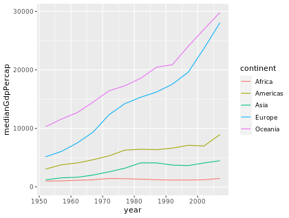
接下来这个例子是根据两个变量year和continent对数据进行组化，求得gdpPercap的中位数，x轴为year，y轴为gdpPercap的中位数进行做图。并且根据continent进行上色。

# Summarize the median gdpPercap by year & continent, save as by_year_continent
by_year_continent<- gapminder %>% 
group_by(year,continent) %>% 
summarize(medianGdpPercap=median(gdpPercap))

# Create a line plot showing the change in medianGdpPercap by continent over time
ggplot(by_year_continent,aes(x=year,y=medianGdpPercap,color=continent))+
geom_line()+
expand_limits(y = 0)

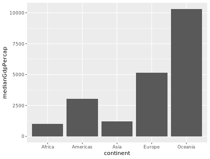
棒状图

选取year为1952的数据，然后根据continent进行组化，计算出gdpPercap的中位数，并对其进行可视化画出棒状图。

# Summarize the median gdpPercap by continent in 1952
by_continent<-gapminder %>% 
filter(year==1952) %>% 
group_by(continent) %>% 
summarize(medianGdpPercap=median(gdpPercap))

# Create a bar plot showing medianGdp by continent
ggplot(by_continent,aes(x=continent,y=medianGdpPercap))+
geom_col()

直方图

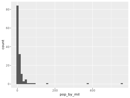
选取年份year为1952的数据，通过pop / 1000000来新增变量pop_by_mil。然后绘制直方图，设置间隔为50。

gapminder_1952 <- gapminder %>%
  filter(year == 1952) %>%
  mutate(pop_by_mil = pop / 1000000)

# Create a histogram of population (pop_by_mil)
ggplot(gapminder_1952,aes(pop_by_mil))+
geom_histogram(bins=50)

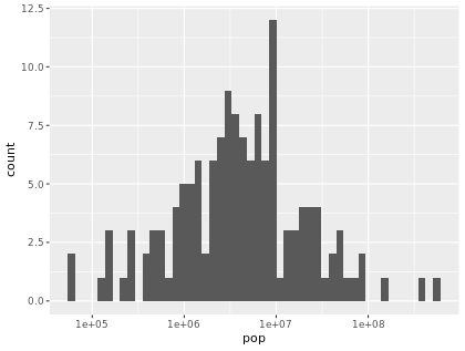
也可以对x轴进行对数转换。选取年份year为1952的数据,画出变量pop的直方图，并对x轴进行对数转换(这是Chapter.1的内容)。

gapminder_1952 <- gapminder %>%
  filter(year == 1952)

# Create a histogram of population (pop), with x on a log scale
ggplot(gapminder_1952,aes(x=pop))+
geom_histogram(bins=50)+
scale_x_log10()

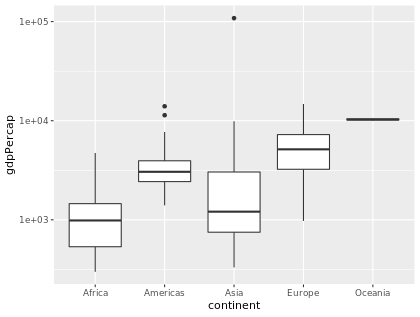
箱图

选取年份为1952的数据，x轴为continent，y轴为gdpPercap画box plot，并对y轴进行对数转换。

gapminder_1952 <- gapminder %>%
  filter(year == 1952)

# Create a boxplot comparing gdpPercap among continents
ggplot(gapminder_1952,aes(x=continent,y=gdpPercap)) +
geom_boxplot()+
scale_y_log10()