回归分析 Python sklearn库 LinearRegression（学习笔记）

#一元回归
import numpy as np
import matplotlib.pyplot as plt
from matplotlib.font_manager import FontProperties
from sklearn.linear_model import LinearRegression

font=FontProperties(fname=r"C:\Windows\Fonts\msyh.ttc",size=15)#设置中文字体

def runplt():
    plt.figure()
    plt.title('身高与体重一元关系',fontproperties=font)
    plt.xlabel('身高（米）',fontproperties=font)
    plt.ylabel('体重（千克）',fontproperties=font)
    plt.axis([0,2,0,85],fontproperties=font)
    plt.grid(True)
    return plt

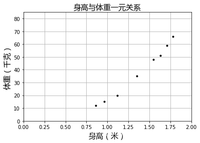
#导入数据，显示
X=[[0.86],[0.96],[1.12],[1.35],[1.55],[1.63],[1.71],[1.78]]
y=[[12],[15],[20],[35],[48],[51],[59],[66]]
plt=runplt()
plt.plot(X,y,'k.')
plt.show()

#训练模型，预测
model=LinearRegression()
model.fit(X,y)
print("预测身高为1.67米的体重是：%.2f千克"%model.predict(np.array([1.67]).reshape(-1,1)))

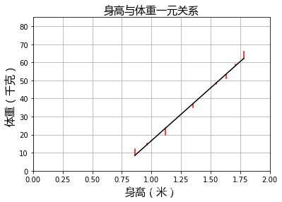
#预测残差
yr=model.predict(X)
plt=runplt()
for idx,x in enumerate(X):
    plt.plot([x,x],[y[idx],yr[idx]],'r-')
plt.plot(X,yr,'k')
plt.show()

预测身高为1.67米的体重是：55.76千克

#预测数据
X2=[[0.75],[1.08],[1.26],[1.51],[1.6],[1.85]]
y_test=[[10],[17],[27],[41],[50],[75]]
y2=model.predict(X2)
plt=runplt()
plt.plot(X2,y2,'g-')
plt.plot(X2,y_test,'k.')
plt.show()
#模型评估
r2=model.score(X2,y_test)
print('R^2=%.2f'%r2)

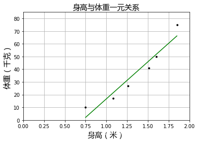
R^2=0.93
可以看出，系数值很高，说明这个一元线性回归模型很好。

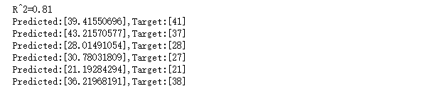
#二元回归
import matplotlib.pyplot as plt
from matplotlib.font_manager import FontProperties
from sklearn.linear_model import LinearRegression

font=FontProperties(fname=r"C:\Windows\Fonts\msyh.ttc",size=15)#设置中文字体

X=[[147,9],[129,7],[141,9],[145,11],[142,11],[151,13]]
y=[[34],[23],[25],[47],[26],[46]]
model=LinearRegression()
model.fit(X,y)#训练模型

X_test=[[149,11],[152,12],[140,8],[138,10],[132,7],[147,10]]
y_test=[[41],[37],[28],[27],[21],[38]]
y_pred=model.predict(X_test)
print('R^2=%.2f'%model.score(X_test,y_test))#模型评估
for i,pred in enumerate(y_pred):
    print("Predicted:%s,Target:%s"%(pred,y_test[i]))

#显示
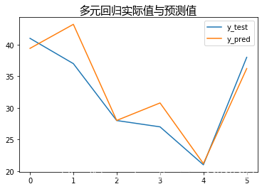
plt.title('多元回归实际值与预测值',fontproperties=font)
plt.plot(y_test,label='y_test')
plt.plot(y_pred,label='y_pred')
plt.legend()
plt.show()

#一元回归预测房价
import pandas as pd
import matplotlib.pyplot as plt
from sklearn.linear_model import LinearRegression

#处理数据，转换成LinearRegression模型可以识别的数据
def get_data(file_name):
    data=pd.read_csv(file_name)
    X_parameter=[]
    Y_parameter=[]
    for value1,value2 in zip(data['square_meter'],data['price']):
        X_parameter.append([float(value1)])
        Y_parameter.append([float(value2)])
    return X_parameter,Y_parameter

#训练模型，预测
def linear_model_main(X_parameter,Y_parameter,pred):
    model=LinearRegression()
    model.fit(X_parameter,Y_parameter)#训练模型
    pred_value=model.predict(pred)#预测
    predictions={}#构造返回字典
    predictions['intercept']=model.intercept_
    predictions['coefficient']=model.coef_
    predictions['predict_value']=pred_value
    return predictions

#图像处理
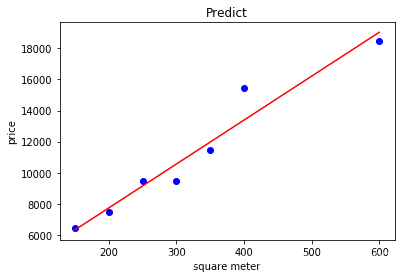
def show_linear_line(X_parameter,Y_parameter):
    model=LinearRegression()
    model.fit(X_parameter,Y_parameter)
    plt.scatter(X_parameter,Y_parameter,color='blue')
    plt.plot(X_parameter,model.predict(X_parameter),color='red')
    plt.title('Predict')
    plt.xlabel('square meter')
    plt.ylabel('price')
    plt.show()
    
#主函数
def main():
    file_name='/house_price.csv'
    X,Y=get_data(file_name)
    pred=[[700]]
    predictions=linear_model_main(X,Y,pred)
    for key,value in predictions.items():
    	print('{0}:{1}'.format(key,value))
    show_linear_line(X,Y)
    
if __name__=='__main__':
    main()

intercept:[2085.63829787]
coefficient:[[28.24468085]]
predict_value:[[21856.91489362]]

#产品销量与广告的多元回归
import pandas as pd
from sklearn.model_selection import train_test_split
from sklearn.linear_model import LinearRegression
import matplotlib.pyplot as plt
from sklearn import metrics
import numpy as np

data=pd.read_csv('/Advertising.csv')
X=data[['TV','radio','newspaper']]
y=data['sales']

#训练集、测试集
X_train,X_test,y_train,y_test=train_test_split(X,y,test_size=0.4,random_state=0)

#训练模型
model=LinearRegression()
model.fit(X_train,y_train)
#print(model)
print("截距:",model.intercept_)
print("斜率:",model.coef_)

#预测
y_pred=model.predict(X_test)
#print(y_pred)

#对比
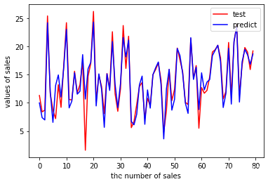
plt.figure()
plt.plot(range(len(y_test)),y_test,'r',label='test')
plt.plot(range(len(y_test)),y_pred,'b',label='predict')
plt.legend(loc='upper right')
plt.xlabel('the number of sales')
plt.ylabel('values of sales')
plt.show()

#模型验证（均方根误差）
sum_mean=0
for i in range(len(y_test)):
    sum_mean+=(y_pred[i]-y_test.values[i])**2
    
sum_erro=np.sqrt(sum_mean/50)
print('RMSE:',sum_erro)

截距: 2.8119370260970715
斜率: [0.04440533 0.19680116 0.00367821]

RMSE: 2.175105361547452