


前言
编码之前是了解我们试图解决的问题和可用的数据。在这个项目中,我们将使用公共可用的纽约市的建筑能源数据。目标是使用能源数据建立一个模型,来预测建筑物的Enerqy Star Score(能源之星分数),并解释结果以找出影响评分的因素。数据包括Eneray Star Score,意味着这是一个监督回归机器学习任务:监督:我们可以知道数据的特征和目标,我们的目标是训练可以学习两者之间映射关系的模型。回归:EnergyStarScore是一个连续变量。我们想要开发一个模型准确性,它可以实现预测EnerayStarScore,并且结果接近真实值。
提示:以下是本篇文章正文内容,下面案例可供参考
一、数据导入、数据清洗与格式转换
import pandas as pd
import numpy as np

# API需要升级或者遗弃了,不想看就设置一下warning
pd.options.mode.chained_assignment = None

# 经常用到head(),最多展示多少条数
pd.set_option('display.max_columns', 60)
import matplotlib.pyplot as plt
%matplotlib inline
#绘图全局的设置好了,画图字体大小
plt.rcParams['font.size'] = 24
from IPython.core.pylabtools import figsize
import seaborn as sns
sns.set(font_scale = 2)
from sklearn.model_selection import train_test_split
import warnings
warnings.filterwarnings("ignore")
二、 数据分析
4.1.2 数据分析
# 加载数据
data = pd.read_csv('data/Energy.csv')
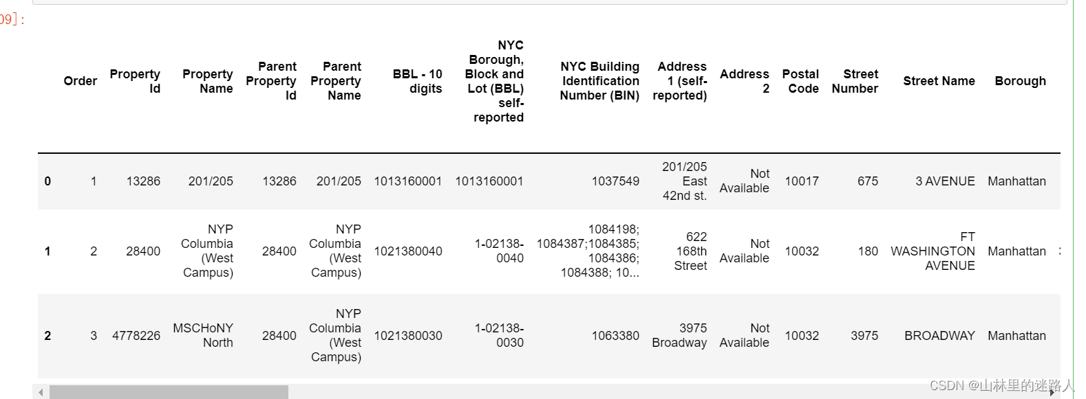
# 展示前3行
data.head(3)
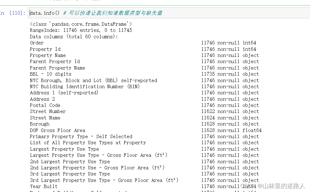
4.1.3 数据类型与缺失值
data.info() # 可以快速让我们知道数据类型与缺失值
缺失值处理模板
4.1. 4 缺失值处理模板
# 缺失值Not Available转换为np.nan
#replace():描述Python replace() 方法把字符串中的 old(旧字符串) 替换成 new(新字符串),
data = data.replace({'Not Available': np.nan})
for col in list(data.columns):
#平方英尺、千英热单位、降低能源成本和温室气体排放、千瓦时、克卡、加仑、得分等结尾的都转化为float类型
if ('ft²' in col or 'kBtu' in col or 'Metric Tons CO2e' in col or 'kWh' in
col or 'therms' in col or 'gal' in col or 'Score' in col):
data[col] = data[col].astype(float)
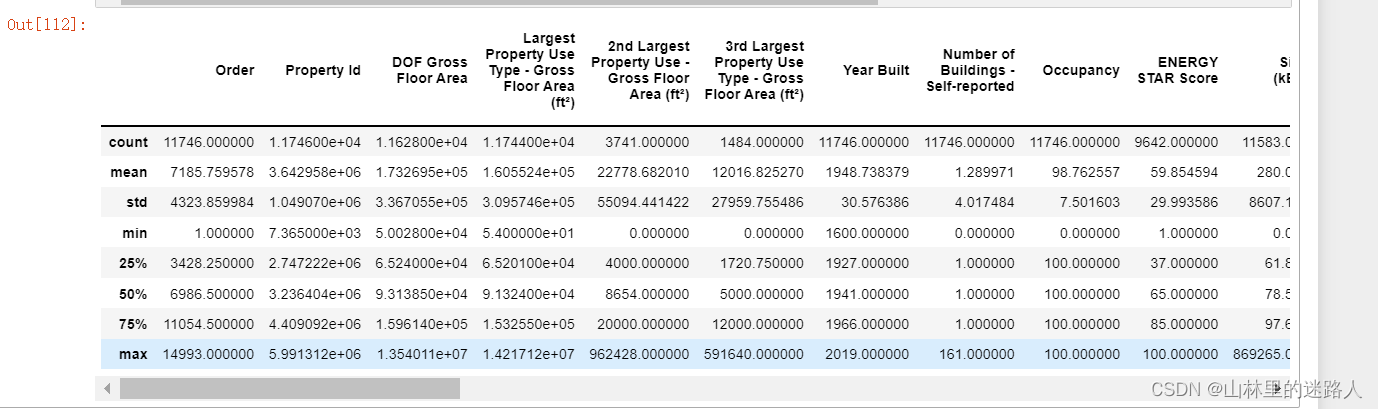
# 每列中只能展示数值型的count、mean、sdt等等,object不会展示
data.describe()
# 3.20e+05=3.20x10^5=3.20x100000=320000
# 在科学计数法中,为了使公式简便,可以用带“E”的格式表示。当用该格式表示时,E前面的数字和“E+”后面要精确到十分位,(位数不够末尾补0),例如7.8乘10的7次方,正常写法为:7.8x10^7,简写为“7.8E+07”的形式
# 缺失值的模板,通用的
#  定义一个函数,传进来一个DataFrame
def missing_values_table(df):
        # python的pandas库中有一个十分便利的isnull()函数,它可以用来判断缺失值,把每列的缺失值算一下总和
        mis_val = df.isnull().sum()

        # 100相当于%,每列的缺失值的占比
        mis_val_percent = 100 * df.isnull().sum() / len(df)

        # 每列缺失值的个数 、 每列缺失值的占比做成表
        mis_val_table = pd.concat([mis_val, mis_val_percent], axis=1)

        # 重命名指定列的名称
        mis_val_table_ren_columns = mis_val_table.rename(
        columns = {0 : 'Missing Values', 1 : '% of Total Values'})

        # 因为第1列缺失值很大,ascending=False代表降序
        #iloc[:,1] != 0的意思是对于下面的表中的第2列(缺失的占比)进行降序,从大到小
        mis_val_table_ren_columns = mis_val_table_ren_columns[
            mis_val_table_ren_columns.iloc[:,1] != 0].sort_values(
        '% of Total Values', ascending=False).round(1)


        print ("Your selected dataframe has " + str(df.shape[1]) + " columns.\n"
            "There are " + str(mis_val_table_ren_columns.shape[0]) +
              " columns that have missing values.")


        return mis_val_table_ren_columns
missing_values_table(data) #第一列是每1列,第二列是缺失值个数,第三列是缺失值%比,一共是60列,有46列是有缺失值
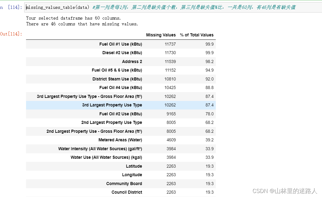
# 50%是阈值,大于50%的列
missing_df = missing_values_table(data);
# 大于50%的列拿出来 ,后面drop()删掉
missing_columns = list(missing_df[missing_df['% of Total Values'] > 50].index)
print('We will remove %d columns.' % len(missing_columns))

#原始的列中有60列,发现有缺失值的列有46列 , 缺失的46列中大于50%的将删除,有11列

# 大于50%的列都drop掉
data = data.drop(columns = list(missing_columns))
Exploratory Data Analysis
4.2.1单变量绘图
figsize(8, 8)
# Y,就是从1~100的能源得分值,重命名为score
data = data.rename(columns = {'ENERGY STAR Score': 'score'})
# 在seaborn中找到不同的风格
plt.style.use('fivethirtyeight')
#dropna():该函数主要用于滤除缺失数据
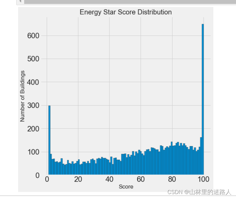
plt.hist(data['score'].dropna(), bins = 100, edgecolor = 'k');
plt.xlabel('Score'); plt.ylabel('Number of Buildings');
plt.title('Energy Star Score Distribution');
#在展示的图中,1和100的得分比较高,原始数据都是物业自己填的报表打得分,根据实际情况,给房屋的能源利用率打的分值,人为填的,
#所以1和100,得分很高,有水分,但是,我们的目标只是预测分数,而不是设计更好的建筑物评分方法! 我们可以在我们的报告中记下分数具有可疑分布,但我们主要关注预测分数。
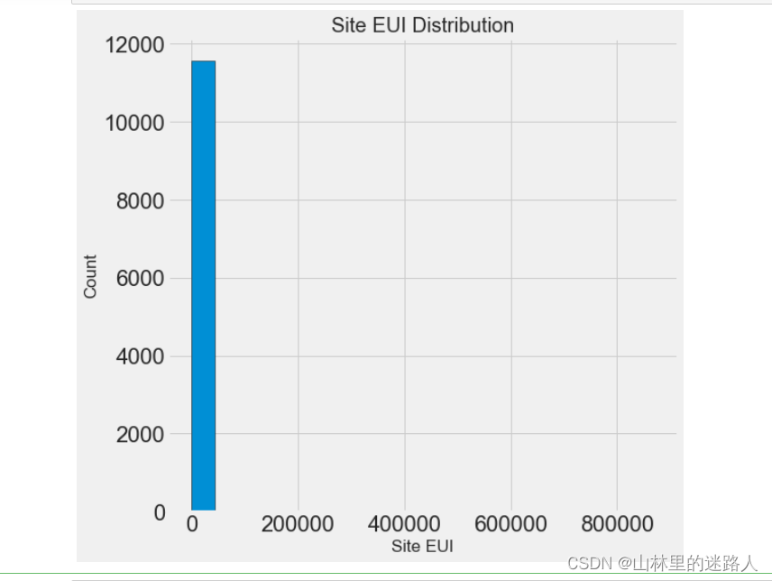
# Site EUI (kBtu/ft²:能源使用强度

figsize(8, 8)
plt.hist(data['Site EUI (kBtu/ft²)'].dropna(), bins = 20, edgecolor = 'black'); # 边也是黑色
plt.xlabel('Site EUI');
plt.ylabel('Count'); plt.title('Site EUI Distribution');

#这显示我们有另一个问题:!由于存在几个非常高分的建筑物,这张图难以置信地倾斜了。所以必须进行异常值处理。
#你会很清楚地看到最后一个值异常大。出现异常值的原因很多:错字,测量设备故障,错误的单位,或者它们可能是合法的但是个极端值
#相当于分一下数据有很多点离均值很远,就有离群点
data['Site EUI (kBtu/ft²)'].describe()
# 均值mean小 , 标准差很大,就意味着有很多点离均值很远,就有离群点 ,因为最小值为0,最大值为869265
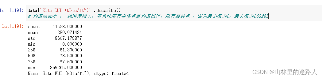
平均值为280,标准差8607,std非常大了,意味着有些数据离大多数围绕均值范围的比较远,最小值为0,最大值为 869265,这才画的很奇怪。
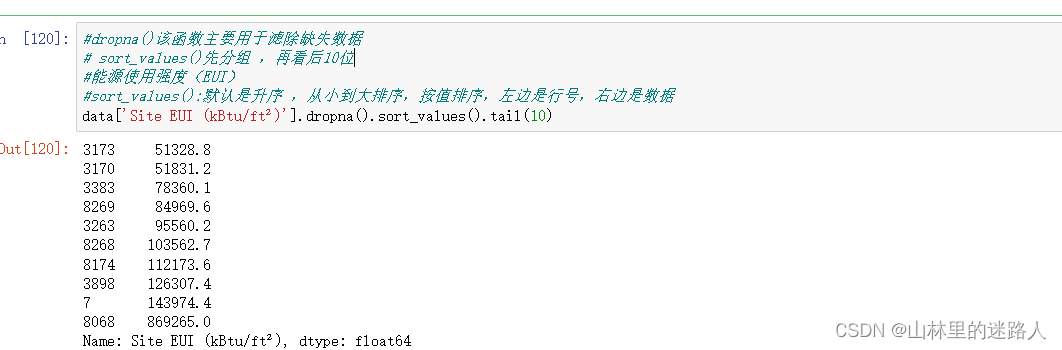
#dropna()该函数主要用于滤除缺失数据
# sort_values()先分组 ,再看后10位
#能源使用强度(EUI)
#sort_values():默认是升序 ,从小到大排序,按值排序,左边是行号,右边是数据
data['Site EUI (kBtu/ft²)'].dropna().sort_values().tail(10)
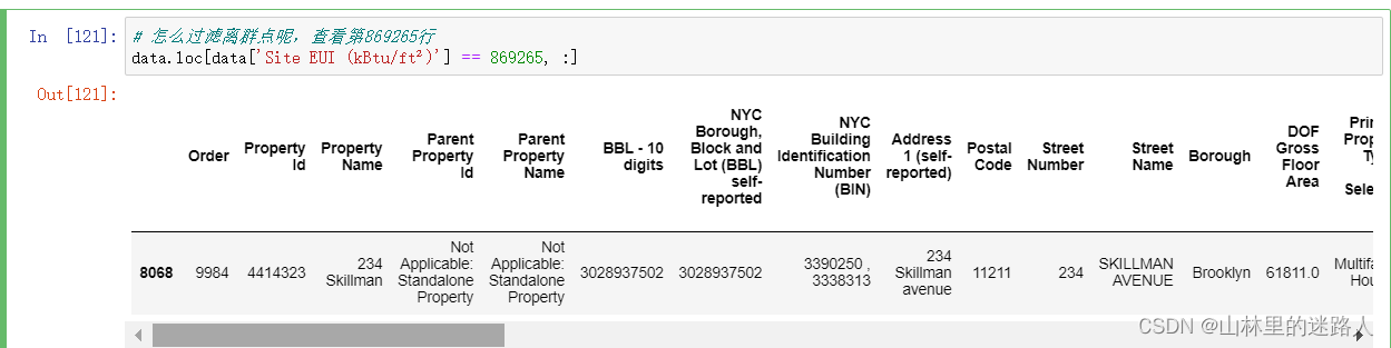
# 怎么过滤离群点呢,查看第869265行
data.loc[data['Site EUI (kBtu/ft²)'] == 869265, :]
剔除离群点
4.2.2剔除离群点
# 在describe取25%和75%分位
first_quartile = data['Site EUI (kBtu/ft²)'].describe()['25%']
third_quartile = data['Site EUI (kBtu/ft²)'].describe()['75%'] # Q3

#  2者一减就是IQ值,就是间隔
iqr = third_quartile - first_quartile


#在这里判断的是正常数据,Q3 - 3IQ  < EUI < Q3+ 3IQ ,保留正常数据,剩下的过滤异常点
# Q3+ 3IQ > 。。。。。。>Q3 - 3IQ ,中间的就是非离群点,就是咱们想要的数据
data = data[(data['Site EUI (kBtu/ft²)'] > (first_quartile - 3 * iqr)) &
            (data['Site EUI (kBtu/ft²)'] < (third_quartile + 3 * iqr))]
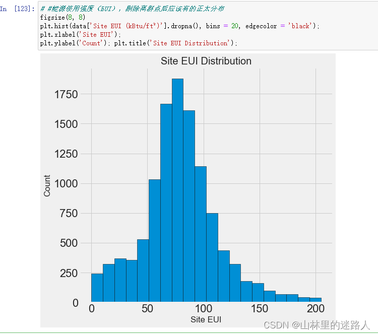
# #能源使用强度(EUI),剔除离群点后应该有的正太分布
figsize(8, 8)
plt.hist(data['Site EUI (kBtu/ft²)'].dropna(), bins = 20, edgecolor = 'black');
plt.xlabel('Site EUI');
plt.ylabel('Count'); plt.title('Site EUI Distribution');
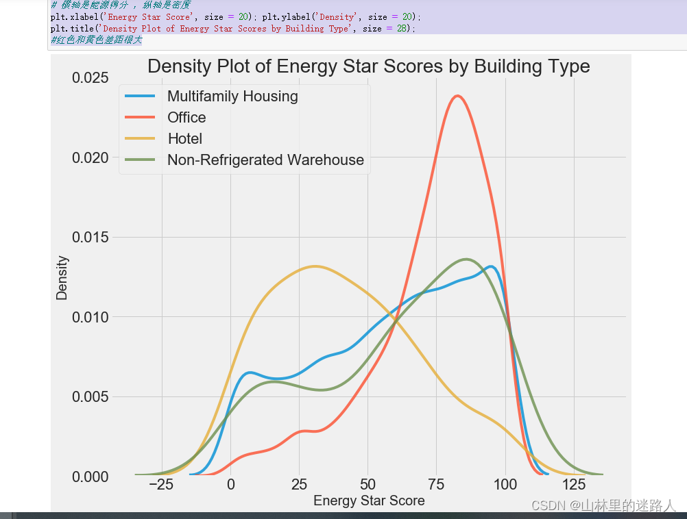
观察哪些变量会对结果产生影响
types = data.dropna(subset=['score'])

#Largest Property Use Type:最大财产使用类型
#该列中有很多的个属性,大于100的值分别有4个属性 , 为:Multifamily Housing——多户住宅区 、 Office——办公室 、 Hotel——酒店
#Data Center, Non-Refrigerated Warehouse, Office——数据中心、非冷藏仓库、办公室

types = types['Largest Property Use Type'].value_counts()
types = list(types[types.values > 100].index)
# 找出差异大的2个选取特征
#Largest Property Use Type:最大财产使用类型/多户家庭的住宅区、办公区、酒店、不制冷的大仓库
figsize(12, 10)

# b_type是变量,types是4种类型
for b_type in types:
    #当前Largest Property Use Type就是画的类型b_type4个 变量
    subset = data[data['Largest Property Use Type'] == b_type]

    # 拿到subset的得分值,alpha指的是透明度
    sns.kdeplot(subset['score'].dropna(),
               label = b_type, shade = False, alpha = 0.8);

# 横轴是能源得分 ,纵轴是密度
plt.xlabel('Energy Star Score', size = 20); plt.ylabel('Density', size = 20);
plt.title('Density Plot of Energy Star Scores by Building Type', size = 28);
#红色和黄色差距很大
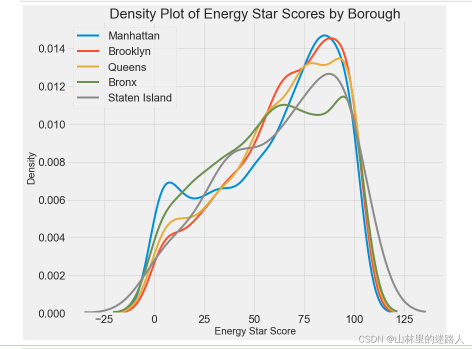
# 查看当前的结果跟地区有什么结果     结果
boroughs = data.dropna(subset=['score'])
#                    地区
boroughs = boroughs['Borough'].value_counts()
boroughs = list(boroughs[boroughs.values > 100].index)
#Borough:自治区镇 ,该列中有5个属性,分别为:Manhattan——曼哈顿 、 Brooklyn——布鲁克林 、 Queens——皇后区 、 Bronx——布朗克斯
# Staten Island——斯塔顿岛


figsize(12, 10)

# 遍历5个属性遍历,画出图,横轴是能源得分、纵轴是密度
for borough in boroughs:

    subset = data[data['Borough'] == borough]


    sns.kdeplot(subset['score'].dropna(),
               label = borough);


plt.xlabel('Energy Star Score', size = 20); plt.ylabel('Density', size = 20);
plt.title('Density Plot of Energy Star Scores by Borough', size = 28);
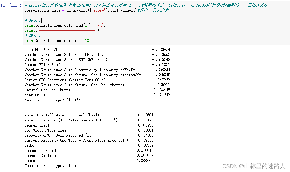
# corr()相关系数矩阵,即给出任意X与Y之间的相关系数 X——>Y两两相关的,负相关多,-0.046605接近于0的都删掉 , 正相关的少
correlations_data = data.corr()['score'].sort_values()#升序,从小到大

# 前10个
print(correlations_data.head(10), '\n')
print("---------------------------")
# 后10个
print(correlations_data.tail(10))
4.3 特征工程
4.3.1 特征变换
import warnings
warnings.filterwarnings("ignore")

# 所有的数值数据拿到手
numeric_subset = data.select_dtypes('number')

# 遍历所有的数值数据
for col in numeric_subset.columns:
    # 如果score就是y值 ,就不做任何变换
    if col == 'score':
        next
    #剩下的不是y的话特征做log和开根号
    else:
        numeric_subset['sqrt_' + col] = np.sqrt(numeric_subset[col])
        numeric_subset['log_' + col] = np.log(numeric_subset[col])

# Borough:自治镇
# Largest Property Use Type:
categorical_subset = data[['Borough', 'Largest Property Use Type']]

# One hot encode用到了读热编码get_dummies
categorical_subset = pd.get_dummies(categorical_subset)


#      合并数组     一个是数值的,      一个热度编码的
features = pd.concat([numeric_subset, categorical_subset], axis = 1)

features = features.dropna(subset = ['score'])

# sort_values()做一下排序
correlations = features.corr()['score'].dropna().sort_values()
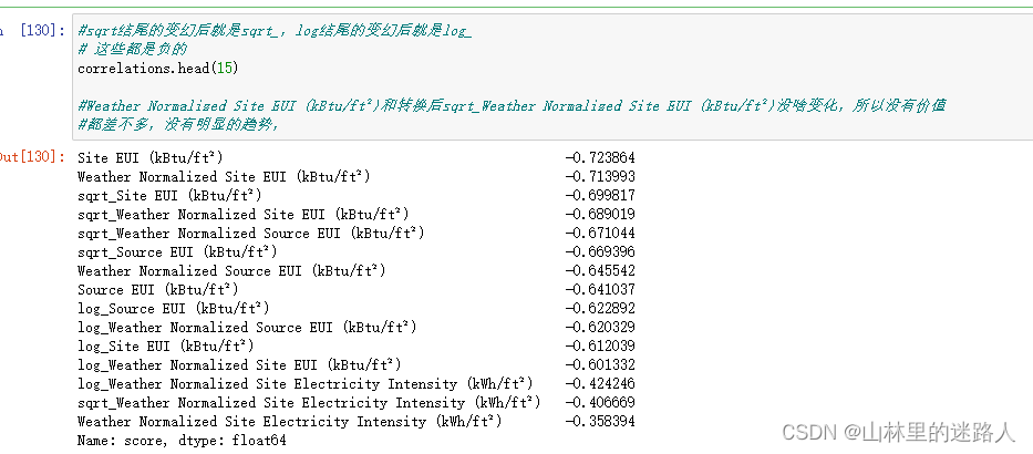
#sqrt结尾的变幻后就是sqrt_,log结尾的变幻后就是log_
# 这些都是负的
correlations.head(15)

#Weather Normalized Site EUI (kBtu/ft²)和转换后sqrt_Weather Normalized Site EUI (kBtu/ft²)没啥变化,所以没有价值
#都差不多,没有明显的趋势,
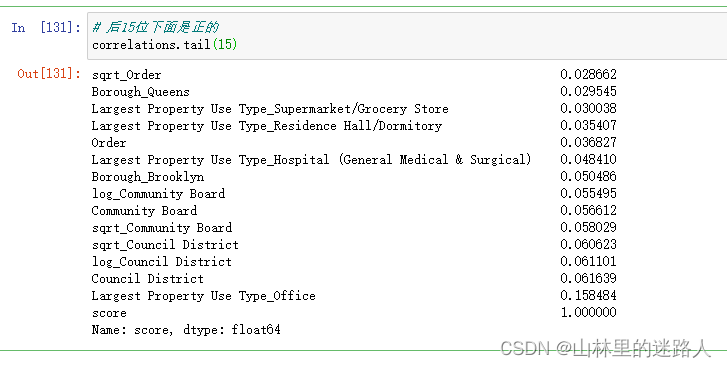
# 后15位下面是正的
correlations.tail(15)
4.3.2 双变量绘图
import warnings
warnings.filterwarnings("ignore")
figsize(12, 10)
# 能源得分与城镇区域之间的关系
features['Largest Property Use Type'] = data.dropna(subset = ['score'])['Largest Property Use Type']
# Largest Property Use Type 最大财产使用类型 ,isin()接受一个列表,判断该列中4个属性是否在列表中
features = features[features['Largest Property Use Type'].isin(types)]
# hue = 'Largest Property Use Type'是4个种类变量 ,4个颜色
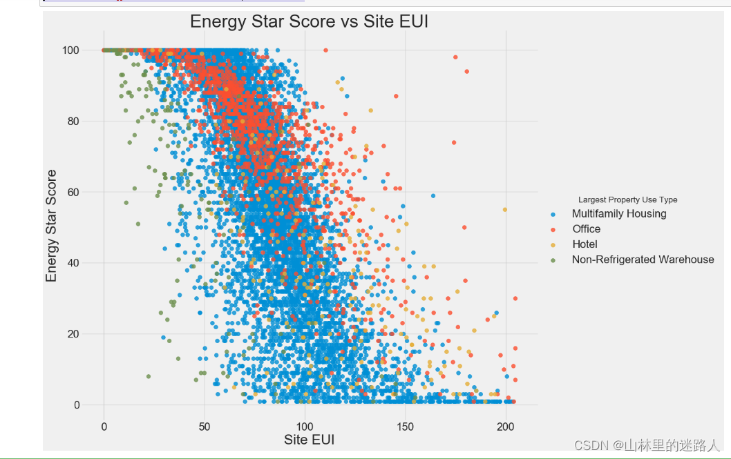
sns.lmplot('Site EUI (kBtu/ft²)', 'score',
# 种类变量,有4个种类,右下角hue是有4个种类变量,
hue = 'Largest Property Use Type', data = features,
scatter_kws = {'alpha': 0.8, 's': 60}, fit_reg = False,
size = 12, aspect = 1.2);
# Plot labeling
plt.xlabel("Site EUI", size = 28)
plt.ylabel('Energy Star Score', size = 28)
plt.title('Energy Star Score vs Site EUI', size = 36);
4.3.3 剔除共线特征
#原始数据备份一下copy(),修改后数据后保持原数据不变
features = data.copy()

# select_dtypes():根据数据类型选择特征,number表示数值型特征
numeric_subset = data.select_dtypes('number')

# 遍历特征是数值型在一个列表中
for col in numeric_subset.columns:
    # 跳过能源得分就是咱们的目标值Y
    if col == 'score':
        next
    else:
        #numeric_subset()从某一个列中选择出符合某条件的数据或是相关的列
        numeric_subset['log_' + col] = np.log(numeric_subset[col])

# Borough:自治区镇
# 最大财产使用类型/多户家庭的a住宅区、办公区、酒店、不制冷的大仓库
categorical_subset = data[['Borough', 'Largest Property Use Type']]


categorical_subset = pd.get_dummies(categorical_subset)

#把所有数值型特征和治区镇以及最大财产的使用类型合并起来
features = pd.concat([numeric_subset, categorical_subset], axis = 1)

features.shape#有110个列,比原来的列多
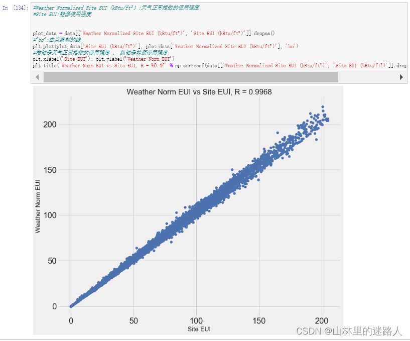
#Weather Normalized Site EUI (kBtu/ft²):天气正常指数的使用强度
#Site EUI:能源使用强度


plot_data = data[['Weather Normalized Site EUI (kBtu/ft²)', 'Site EUI (kBtu/ft²)']].dropna()
#'bo':由点绘制的线
plt.plot(plot_data['Site EUI (kBtu/ft²)'], plot_data['Weather Normalized Site EUI (kBtu/ft²)'], 'bo')
#横轴是天气正常指数的使用强度 、 纵轴是能源使用强度
plt.xlabel('Site EUI'); plt.ylabel('Weather Norm EUI')
plt.title('Weather Norm EUI vs Site EUI, R = %0.4f' % np.corrcoef(data[['Weather Normalized Site EUI (kBtu/ft²)', 'Site EUI (kBtu/ft²)']].dropna(), rowvar=False)[0][1]);
def remove_collinear_features(x, threshold):
    y = x['score'] #在原始数据X中”score“当做y值
    x = x.drop(columns = ['score']) #除去标签值以外的当做特征
    # 多长运行,直到相关性小于阈值才稳定结束
    while True:
        # 计算一个矩阵 ,两两的相关系数
        corr_matrix = x.corr()

        for i in range(len(corr_matrix)):
            corr_matrix.iloc[i][i] = 0 # 将对角线上的相关系数置为0。避免自己跟自己计算相关系数一定大于阈值

        # 定义待删除的特征。
        drop_cols = []
        # col返回的是列名


        for col in corr_matrix:
            if col not in drop_cols: # A和B比 ,B和A比的相关系数一样,避免AB全删了
                # 取相关系数的绝对值。
                v = np.abs(corr_matrix[col]) # 取的是每一列的相关系数
                # 如果相关系数大于设置的阈值
                if np.max(v) > threshold:
                    # 取出最大值对应的索引。
                    name = np.argmax(v) # 找到最大值的的列名
                    drop_cols.append(name)
         # 列表不为空,就删除,列表为空,符合条件,退出循环
        if drop_cols:
            # 删除想删除的列
            x = x.drop(columns=drop_cols, axis=1)
        else:
            break

    # 指定标签
    x['score'] = y

    return x
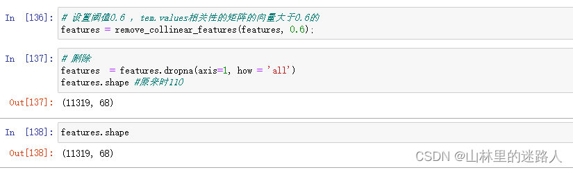
# 设置阈值0.6 ,tem.values相关性的矩阵的向量大于0.6的
features = remove_collinear_features(features, 0.6);
# 删除
features  = features.dropna(axis=1, how = 'all')
features.shape #原来时110
features.shape
4.4 分割数据集
4.4.1 划分数据
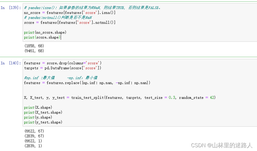
# pandas:isna(): 如果参数的结果为#NaN, 则结果TRUE, 否则结果是FALSE。
no_score = features[features['score'].isna()]
# pandas:notnull()判断是否不是NaN
score = features[features['score'].notnull()]

print(no_score.shape)
print(score.shape)
features = score.drop(columns='score')
targets = pd.DataFrame(score['score'])

#np.inf :最大值      -np.inf:最小值
features = features.replace({np.inf: np.nan, -np.inf: np.nan})


X, X_test, y, y_test = train_test_split(features, targets, test_size = 0.3, random_state = 42)

print(X.shape)
print(X_test.shape)
print(y.shape)
print(y_test.shape)
4.4.2 建立Baseline
# mae平均的绝对值 ,就是 (真实值 - 预测值) / n
#abs():绝对值
def mae(y_true, y_pred):
    return np.mean(abs(y_true - y_pred))
baseline_guess = np.median(y)

print('The baseline guess is a score of %0.2f' % baseline_guess) # 中位数为66
print("Baseline Performance on the test set: MAE = %0.4f" % mae(y_test, baseline_guess)) # MAE = 24.5164

4.4.3 结果保存下来,建模再用
# Save the no scores, training, and testing data
no_score.to_csv('data/no_score.csv', index = False)
X.to_csv('data/training_features.csv', index = False)
X_test.to_csv('data/testing_features.csv', index = False)
y.to_csv('data/training_labels.csv', index = False)
y_test.to_csv('data/testing_labels.csv', index = False)
4.5 建立基础模型,尝试多种算法
#之前把精力都放在了前面了,这回我的重点就要放在建模上了,导入所需要的包
# 数据分析库
import pandas as pd
import numpy as np

# warnings:警告——>忽视
pd.options.mode.chained_assignment = None
pd.set_option('display.max_columns', 60)

# 可视化
import matplotlib.pyplot as plt
%matplotlib inline

# 字体大小设置
plt.rcParams['font.size'] = 24

from IPython.core.pylabtools import figsize

# Seaborn 高级可视化工具
import seaborn as sns
sns.set(font_scale = 2)

# 预处理:缺失值 、 最大最小归一化
from sklearn.preprocessing import Imputer, MinMaxScaler

# 机器学习算法库
from sklearn.linear_model import LinearRegression
from sklearn.ensemble import RandomForestRegressor, GradientBoostingRegressor
from sklearn.svm import SVR
from sklearn.neighbors import KNeighborsRegressor

# 调参工具包
from sklearn.model_selection import RandomizedSearchCV, GridSearchCV


import warnings
warnings.filterwarnings("ignore")
上次保存好的数据加载进来
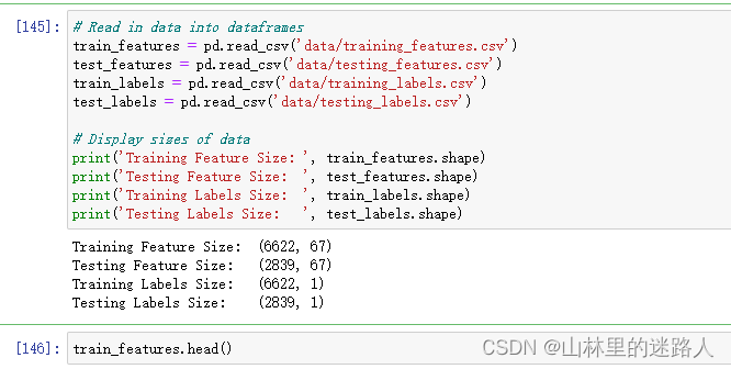
# Read in data into dataframes
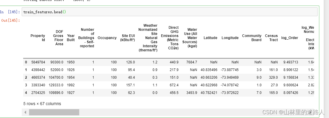
train_features = pd.read_csv('data/training_features.csv')
test_features = pd.read_csv('data/testing_features.csv')
train_labels = pd.read_csv('data/training_labels.csv')
test_labels = pd.read_csv('data/testing_labels.csv')
# Display sizes of data
print('Training Feature Size: ', train_features.shape)
print('Testing Feature Size: ', test_features.shape)
print('Training Labels Size: ', train_labels.shape)
print('Testing Labels Size: ', test_labels.shape)
4.5.1 缺失值填充
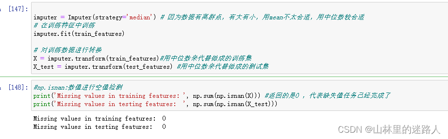
imputer = Imputer(strategy='median') # 因为数据有离群点,有大有小,用mean不太合适,用中位数较合适
# 在训练特征中训练
imputer.fit(train_features)

# 对训练数据进行转换
X = imputer.transform(train_features)#用中位数来代替做成的训练集
X_test = imputer.transform(test_features) #用中位数来代替做成的测试集
#np.isnan:数值进行空值检测
print('Missing values in training features: ', np.sum(np.isnan(X))) #返回的是0 ,代表缺失值任务已经完成了
print('Missing values in testing features:  ', np.sum(np.isnan(X_test)))
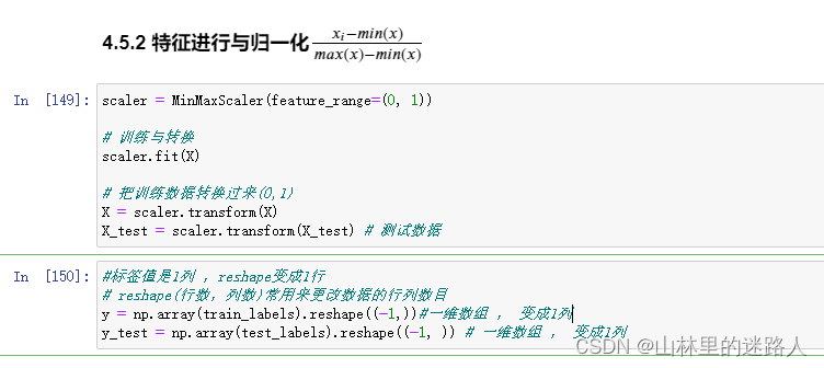
4.5.2 特征进行与归一化 x i − m i n ( x ) m a x ( x ) − m i n ( x ) \frac{x_i - min(x)}{max(x) - min(x)} max(x)−min(x)xi−min(x)
scaler = MinMaxScaler(feature_range=(0, 1))

# 训练与转换
scaler.fit(X)

# 把训练数据转换过来(0,1)
X = scaler.transform(X)
X_test = scaler.transform(X_test) # 测试数据
#标签值是1列 ,reshape变成1行
# reshape(行数,列数)常用来更改数据的行列数目
y = np.array(train_labels).reshape((-1,))#一维数组 , 变成1列
y_test = np.array(test_labels).reshape((-1, )) # 一维数组 , 变成1列
4.6 建立基础模型,尝试多种算法(回归问题)

4.6.1 建立损失函数
# 在这里的损失函数是MAE ,abs()是绝对值
def mae(y_true, y_pred):
    return np.mean(abs(y_true - y_pred))


#制作一个模型 ,训练模型和在验证集上验证模型的参数
def fit_and_evaluate(model):

    # 训练模型
    model.fit(X, y)

    # 训练模型开始在测试数据上训练
    model_pred = model.predict(X_test)
    model_mae = mae(y_test, model_pred)


    return model_mae
4.6.2 选择机器学习算法
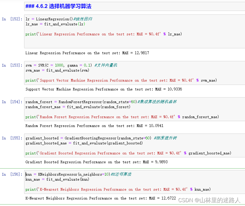
lr = LinearRegression()#线性回归
lr_mae = fit_and_evaluate(lr)

print('Linear Regression Performance on the test set: MAE = %0.4f' % lr_mae)
svm = SVR(C = 1000, gamma = 0.1) #支持向量机
svm_mae = fit_and_evaluate(svm)

print('Support Vector Machine Regression Performance on the test set: MAE = %0.4f' % svm_mae)
random_forest = RandomForestRegressor(random_state=60)#集成算法的随机森林
random_forest_mae = fit_and_evaluate(random_forest)

print('Random Forest Regression Performance on the test set: MAE = %0.4f' % random_forest_mae)
gradient_boosted = GradientBoostingRegressor(random_state=60) #梯度提升树
gradient_boosted_mae = fit_and_evaluate(gradient_boosted)

print('Gradient Boosted Regression Performance on the test set: MAE = %0.4f' % gradient_boosted_mae)
knn = KNeighborsRegressor(n_neighbors=10)#K近邻算法
knn_mae = fit_and_evaluate(knn)

print('K-Nearest Neighbors Regression Performance on the test set: MAE = %0.4f' % knn_mae)
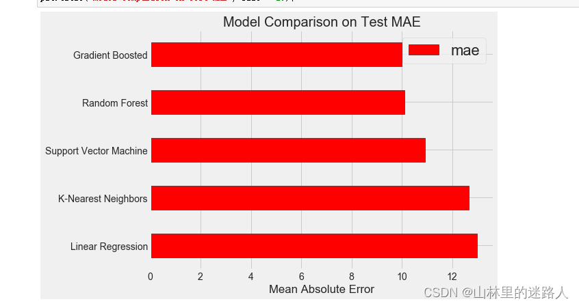
plt.style.use('fivethirtyeight')
figsize(8, 6)


model_comparison = pd.DataFrame({'model': ['Linear Regression', 'Support Vector Machine',
                                           'Random Forest', 'Gradient Boosted',
                                            'K-Nearest Neighbors'],
                                 'mae': [lr_mae, svm_mae, random_forest_mae,
                                         gradient_boosted_mae, knn_mae]})

#         ascending=True是对的意思升序      降序 :从大到小/从第1行到第5行    barh:横着去画的直方图
model_comparison.sort_values('mae', ascending = False).plot(x = 'model', y = 'mae', kind = 'barh',
                                                           color = 'red', edgecolor = 'black')

# 纵轴是算法模型的名称    yticks:为递增值向量       横轴是MAE损失                 xticks:为递增值向量
plt.ylabel(''); plt.yticks(size = 14); plt.xlabel('Mean Absolute Error'); plt.xticks(size = 14)
plt.title('Model Comparison on Test MAE', size = 20);
4.7 模型调参
loss = ['ls', 'lad', 'huber']

# 所使用的弱“学习者”(决策树)的数量
n_estimators = [100, 500, 900, 1100, 1500]

# 决策树的最大深度
max_depth = [2, 3, 5, 10, 15]

# 决策树的叶节点所需的最小示例个数
min_samples_leaf = [1, 2, 4, 6, 8]

# 分割决策树节点所需的最小示例个数
min_samples_split = [2, 4, 6, 10]


hyperparameter_grid = {'loss': loss,
                       'n_estimators': n_estimators,
                       'max_depth': max_depth,
                       'min_samples_leaf': min_samples_leaf,
                       'min_samples_split': min_samples_split}
model = GradientBoostingRegressor(random_state = 42)


random_cv = RandomizedSearchCV(estimator=model,

                               param_distributions=hyperparameter_grid,
                               cv=4, n_iter=25,
                               scoring = 'neg_mean_absolute_error', #选择好结果的评估值

                               n_jobs = -1, verbose = 1,

                               return_train_score = True,

                               random_state=42)
# 注意:运行的时间非常慢,需要14mins
random_cv.fit(X, y)
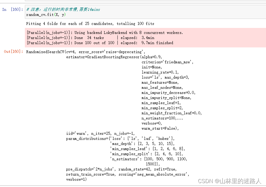
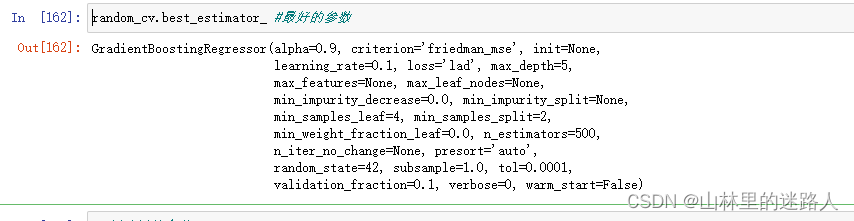
random_cv.best_estimator_ #最好的参数
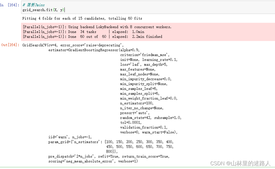
# 创建树策个数
trees_grid = {'n_estimators': [100, 150, 200, 250, 300, 350, 400, 450, 500, 550, 600, 650, 700, 750, 800]}

#建立模型
#lad:最小化绝对偏差
model = GradientBoostingRegressor(loss = 'lad', max_depth = 5,
                                  min_samples_leaf = 6,
                                  min_samples_split = 6,
                                  max_features = None,
                                  random_state = 42)

# 传入参数
grid_search = GridSearchCV(estimator = model, param_grid=trees_grid, cv = 4,
                           scoring = 'neg_mean_absolute_error', verbose = 1,
                           n_jobs = -1, return_train_score = True)
# 需要3mins
grid_search.fit(X, y)
4.7.2 对比损失函数
# 得到结果传入DataFrame
results = pd.DataFrame(grid_search.cv_results_)
# 画图操作
figsize(8, 8)
plt.style.use('fivethirtyeight')
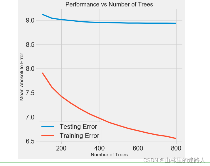
plt.plot(results['param_n_estimators'], -1 * results['mean_test_score'], label = 'Testing Error')
plt.plot(results['param_n_estimators'], -1 * results['mean_train_score'], label = 'Training Error')
#横轴是树的个数 ,纵轴是MAE的误差
plt.xlabel('Number of Trees'); plt.ylabel('Mean Abosolute Error'); plt.legend();
plt.title('Performance vs Number of Trees');
#过拟合 , 蓝色平缓 ,红色比较陡 ,中间的数据越来陡,所以overfiting
4.8 评估与测试:预测和真实之间的差异图
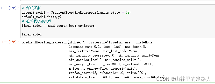
# 测试模型
default_model = GradientBoostingRegressor(random_state = 42)
default_model.fit(X,y)
# 选择最好的参数
final_model = grid_search.best_estimator_

final_model
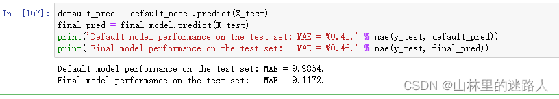
default_pred = default_model.predict(X_test)
final_pred = final_model.predict(X_test)
print('Default model performance on the test set: MAE = %0.4f.' % mae(y_test, default_pred))
print('Final model performance on the test set:   MAE = %0.4f.' % mae(y_test, final_pred))
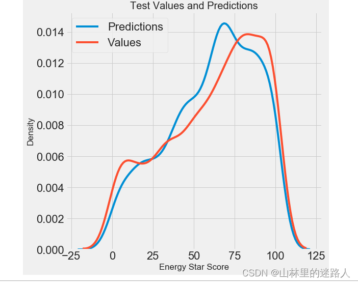
figsize(8, 8)
sns.kdeplot(final_pred, label = 'Predictions')
sns.kdeplot(y_test, label = 'Values')


plt.xlabel('Energy Star Score'); plt.ylabel('Density');
plt.title('Test Values and Predictions');
figsize = (6, 6)
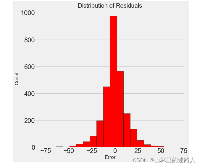
# 最终的模型差异 = 模型 - 测试值 ,大部分都在+-25%
residuals = final_pred - y_test
plt.hist(residuals, color = 'red', bins = 20,
edgecolor = 'black')
plt.xlabel('Error'); plt.ylabel('Count')
plt.title('Distribution of Residuals');
4.9 解释模型:基于重要性来进行特征选择
import pandas as pd
import numpy as np


pd.options.mode.chained_assignment = None
pd.set_option('display.max_columns', 60)


import matplotlib.pyplot as plt
%matplotlib inline


plt.rcParams['font.size'] = 24

from IPython.core.pylabtools import figsize

import seaborn as sns

sns.set(font_scale = 2)


from sklearn.preprocessing import Imputer, MinMaxScaler

from sklearn.linear_model import LinearRegression
from sklearn.ensemble import GradientBoostingRegressor

from sklearn import tree


import warnings
warnings.filterwarnings("ignore")
train_features = pd.read_csv('data/training_features.csv')
test_features = pd.read_csv('data/testing_features.csv')
train_labels = pd.read_csv('data/training_labels.csv')
test_labels = pd.read_csv('data/testing_labels.csv')
# 用中值代替缺失值
imputer = Imputer(strategy='median')

# 开始训练
imputer.fit(train_features)


X = imputer.transform(train_features)
X_test = imputer.transform(test_features)


y = np.array(train_labels).reshape((-1,))
y_test = np.array(test_labels).reshape((-1,))
def mae(y_true, y_pred):
    return np.mean(abs(y_true - y_pred))
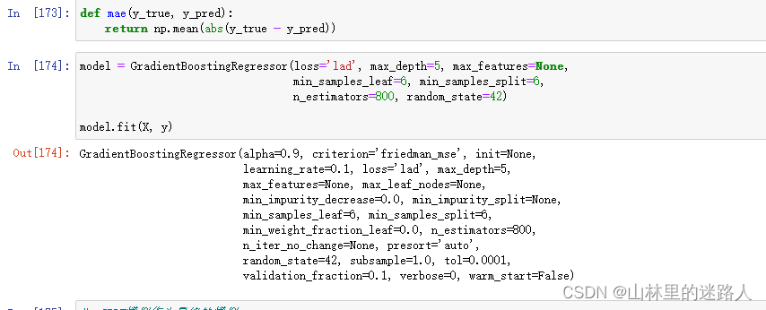
model = GradientBoostingRegressor(loss='lad', max_depth=5, max_features=None,
                                  min_samples_leaf=6, min_samples_split=6,
                                  n_estimators=800, random_state=42)

model.fit(X, y)
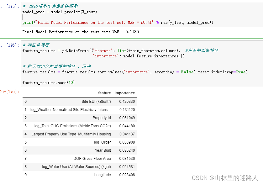
#  GBDT模型作为最终的模型
model_pred = model.predict(X_test)

print('Final Model Performance on the test set: MAE = %0.4f' % mae(y_test, model_pred))
# 特征重要度
feature_results = pd.DataFrame({'feature': list(train_features.columns),  #所有的训练特征
                                'importance': model.feature_importances_})

# 展示前10名的重要的特征 ,降序
feature_results = feature_results.sort_values('importance', ascending = False).reset_index(drop=True)

feature_results.head(10)
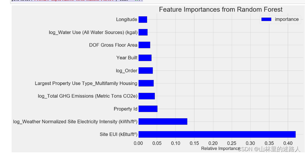
figsize(12, 10)
plt.style.use('fivethirtyeight')

# 展示前10名的重要的特征
feature_results.loc[:9, :].plot(x = 'feature', y = 'importance',
                                 edgecolor = 'k',
                                 kind='barh', color = 'blue');#barh:直方图横着
plt.xlabel('Relative Importance', size = 20); plt.ylabel('')
plt.title('Feature Importances from Random Forest', size = 30);
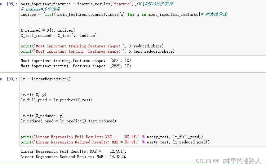
most_important_features = feature_results['feature'][:10]#前10行的特征
# indices=10个列名
indices = [list(train_features.columns).index(x) for x in most_important_features]# 列表推导式


X_reduced = X[:, indices]
X_test_reduced = X_test[:, indices]

print('Most important training features shape: ', X_reduced.shape)
print('Most important testing  features shape: ', X_test_reduced.shape)
lr = LinearRegression()


lr.fit(X, y)
lr_full_pred = lr.predict(X_test)


lr.fit(X_reduced, y)
lr_reduced_pred = lr.predict(X_test_reduced)


print('Linear Regression Full Results: MAE =    %0.4f.' % mae(y_test, lr_full_pred))
print('Linear Regression Reduced Results: MAE = %0.4f.' % mae(y_test, lr_reduced_pred))


 1万+
1万+


 被折叠的 条评论
为什么被折叠?
被折叠的 条评论
为什么被折叠?
 到【灌水乐园】发言


