python小波分析

基于python进行小波分析，频率谱分析_python 频谱分配-CSDN博客

python小波分析，频率普分析——代码修改_sunny_xx.的博客-CSDN博客
wavelets/wave_python at master · chris-torrence/wavelets · GitHub
https://github.com/chris-torrence/wavelets/tree/master/wave_python

以上借鉴前人经验

python代码

import sys

# 添加指定目录到模块搜索路径
module_path = r'F:\A 毕业论文\original data\waveletAnalysis'
sys.path.append(module_path)

# 现在可以导入子目录中的模块
from waveletFunctions import wavelet, wave_signif
import numpy as np
import matplotlib.pylab as plt
from matplotlib.gridspec import GridSpec
import matplotlib.ticker as ticker
from mpl_toolkits.axes_grid1 import make_axes_locatable

# READ THE DATA
sst = np.loadtxt('F:\\A 毕业论文\\original data\\waveletAnalysis\\sst_nino3.dat')  # input SST time series
sst = sst - np.mean(sst)
variance = np.std(sst, ddof=1) ** 2
print("variance = ", variance)

if 0:
    variance = 1.0
    sst = sst / np.std(sst, ddof=1)
n = len(sst)
dt = 0.25
time = np.arange(len(sst)) * dt + 1980.0  # construct time array
xlim = ([1980, 2022])  # plotting range
pad = 1  # pad the time series with zeroes (recommended)
dj =0.25  # this will do 4 sub-octaves per octave
s0 = 2 * dt  # this says start at a scale of 6 months
j1 = 7 / dj  # this says do 7 powers-of-two with dj sub-octaves each
lag1 = 0.72  # lag-1 autocorrelation for red noise background
print("lag1 = ", lag1)
mother = 'MORLET'

# Wavelet transform:
wave, period, scale, coi = wavelet(sst, dt, pad, dj, s0, j1, mother)
power = (np.abs(wave)) ** 2  # compute wavelet power spectrum
global_ws = (np.sum(power, axis=1) / n)  # time-average over all times

# Significance levels:
signif = wave_signif(([variance]), dt=dt, sigtest=0, scale=scale,
    lag1=lag1, mother=mother)
sig95 = signif[:, np.newaxis].dot(np.ones(n)[np.newaxis, :])  # expand signif --> (J+1)x(N) array
sig95 = power / sig95  # where ratio > 1, power is significant

# Global wavelet spectrum & significance levels:
dof = n - scale  # the -scale corrects for padding at edges
global_signif = wave_signif(variance, dt=dt, scale=scale, sigtest=1,
    lag1=lag1, dof=dof, mother=mother)

# Scale-average between El Nino periods of 2--8 years
avg = np.logical_and(scale >= 2, scale < 8)
Cdelta = 0.776  # this is for the MORLET wavelet
scale_avg = scale[:, np.newaxis].dot(np.ones(n)[np.newaxis, :])  # expand scale --> (J+1)x(N) array
scale_avg = power / scale_avg  # [Eqn(24)]
scale_avg = dj * dt / Cdelta * sum(scale_avg[avg, :])  # [Eqn(24)]
scaleavg_signif = wave_signif(variance, dt=dt, scale=scale, sigtest=2,
    lag1=lag1, dof=([2, 7.9]), mother=mother)

#------------------------------------------------------ Plotting

#--- Plot time series
fig = plt.figure(figsize=(9, 10))
gs = GridSpec(3, 4, hspace=0.4, wspace=0.75)
plt.subplots_adjust(left=0.1, bottom=0.05, right=0.9, top=0.95, wspace=0, hspace=0)
plt.subplot(gs[0, 0:3])
plt.plot(time, sst, 'k')
plt.xlim(xlim[:])
plt.xlabel('Time (year)')
plt.ylabel('dust concentration ( μg/m³)')
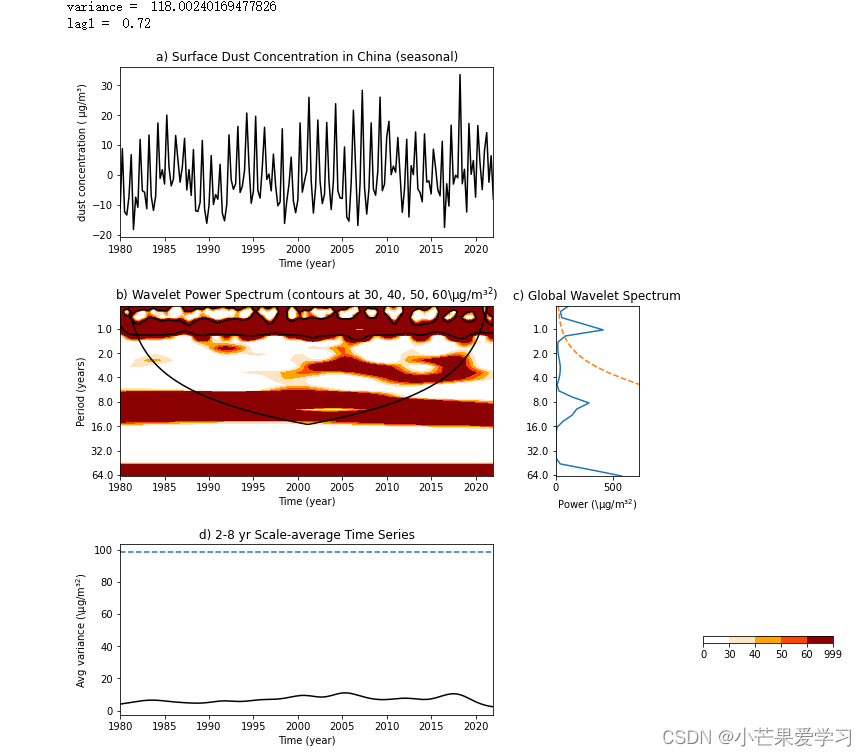
plt.title('a) Surface Dust Concentration in China (seasonal)')

#--- Contour plot wavelet power spectrum
# plt3 = plt.subplot(3, 1, 2)
plt3 = plt.subplot(gs[1, 0:3])
levels = [0, 30, 40, 50, 60, 999]
CS = plt.contourf(time, period, power, len(levels))  #*** or use 'contour'
im = plt.contourf(CS, levels=levels, colors=['white','bisque','orange','orangered','darkred'])
plt.xlabel('Time (year)')
plt.ylabel('Period (years)')
plt.title('b) Wavelet Power Spectrum (contours at 30, 40, 50, 60\μg/m³$^2$)')
plt.xlim(xlim[:])
# 95# significance contour, levels at -99 (fake) and 1 (95# signif)
plt.contour(time, period, sig95, [-99, 1], colors='k')
# cone-of-influence, anything "below" is dubious
plt.plot(time, coi, 'k')
# format y-scale
plt3.set_yscale('log', base=2
                )
plt.ylim([np.min(period), np.max(period)])
ax = plt.gca().yaxis
ax.set_major_formatter(ticker.ScalarFormatter())
plt3.ticklabel_format(axis='y', style='plain')
plt3.invert_yaxis()


# set up the size and location of the colorbar
position=fig.add_axes([1,0.15,0.2,0.01]) ##颜色条位置
plt.colorbar(im, cax=position, orientation='horizontal') #, fraction=0.05, pad=0.5)

# plt.subplots_adjust(right=0.7, top=0.9)

#--- Plot global wavelet spectrum
plt4 = plt.subplot(gs[1, -1])
plt.plot(global_ws, period)
plt.plot(global_signif, period, '--')
plt.xlabel('Power (\μg/m³$^2$)')
plt.title('c) Global Wavelet Spectrum')
plt.xlim([0, 1.25 * np.max(global_ws)])
# format y-scale
plt4.set_yscale('log', base=2)
plt.ylim([np.min(period), np.max(period)])
ax = plt.gca().yaxis
ax.set_major_formatter(ticker.ScalarFormatter())
plt4.ticklabel_format(axis='y', style='plain')
plt4.invert_yaxis()

# --- Plot 2--8 yr scale-average time series
plt.subplot(gs[2, 0:3])
plt.plot(time, scale_avg, 'k')
plt.xlim(xlim[:])
plt.xlabel('Time (year)')
plt.ylabel('Avg variance (\μg/m³$^2$)')
plt.title('d) 2-8 yr Scale-average Time Series')
plt.plot(xlim, scaleavg_signif + [0, 0], '--')

plt.show()

# end of codeimport matplotlib as mpl

结果图