


人工智能三学派
行为主义:感知-动作的控制系统
符号主义:用公式描述、理性思维
连接主义:感性思维(神经网络)
神经网络设计过程
给鸢尾花分类
通过测量花的花萼长、花萼宽、花瓣长、花瓣宽得出鸢尾花的类别
1、if语句 case语句——专家系统:把专家的经验告知计算机,计算机执行逻辑判别给出分类(符号主义)
2、神经网络:采集大量数据对(输入特征,标签)构成数据集,构建网络,梯度下降,反向传播
反向传播
import tensorflow as tf
w = tf.Variable(tf.constant(5, dtype=tf.float32))
lr = 0.2
epoch = 40
for epoch in range(epoch): # for epoch 定义顶层循环,表示对数据集循环epoch次,此例数据集数据仅有1个w,初始化时候constant赋值为5,循环40次迭代。
with tf.GradientTape() as tape: # with结构到grads框起了梯度的计算过程。
loss = tf.square(w + 1)
grads = tape.gradient(loss, w) # .gradient函数告知谁对谁求导
w.assign_sub(lr * grads) # .assign_sub 对变量做自减 即:w -= lr*grads 即 w = w - lr*grads
print("After %s epoch,w is %f,loss is %f" % (epoch, w.numpy(), loss))
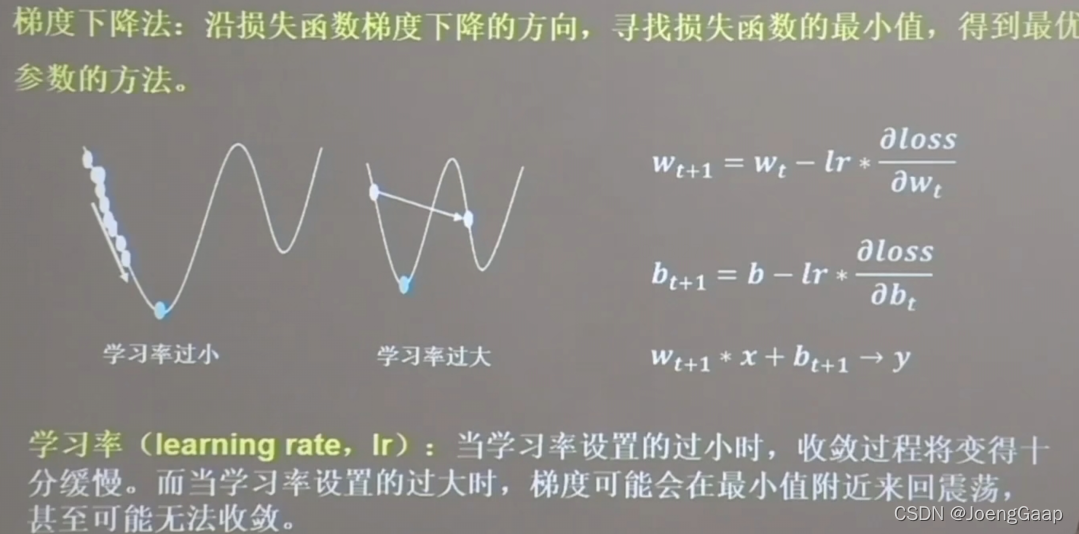
# lr初始值:0.2 请自改学习率 0.001 0.999 看收敛过程
# 最终目的:找到 loss 最小 即 w = -1 的最优参数w
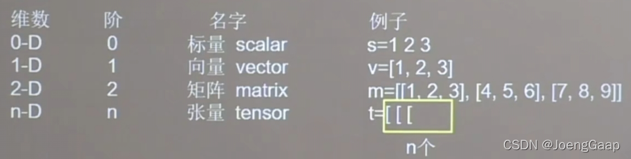
张量生成
张量(Tensor):多维数组(列表) 阶:张量的维数
数据类型
tf.int ,tf.float ,…
tf.int32, tf.float32, tf.float64
tf.bool
tf.constant([True,False])
tf,string
tf.constant(“Hello,world!”)
创建一个张量
tf.constant(张量内容,dtype=数据类型(可选))
import tensorflow as tf
a=tf.constant([1,5],dtype=tf.int64)#[1,5]是张量内容也就是一阶张量的值是1,5,不是张量大小
print(a)
print(a.dtype)
print(a.shape)
运行结果:
tf.Tensor([1 5], shape=(2,), dtype=int64)#shape隔开了几个数字就是几维的,这里是一维的
<dtype: 'int64'>
(2,)
将numpy的数据类型转换为Tensor数据类型
tf.convert_to_tensor(数据名,dtype=数据类型(可选))
import tensorflow as tf
import numpy as np
a=np.arange(0,5)
b=tf.convert_to_tensor(a,dtype=tf.int64)
print(a)
print(b)
[0 1 2 3 4]
tf.Tensor([0 1 2 3 4], shape=(5,), dtype=int64)
创建全为0的张量
tf.zeros(维度)
创建全为1的张量
tf.ones(维度)
创建全为指定值的张量
tf.fill(维度,指定值)
维度:
一维 直接写个数
二维 用[行,列]
多维 用[n,m,j,k,…]
import tensorflow as tf
a=tf.zeros([2,3])
b=tf.ones(4)
c=tf.fill([2,2],9)
print(a)
print(b)
print(c)
运行结果:
tf.Tensor(
[[0. 0. 0.]
 [0. 0. 0.]], shape=(2, 3), dtype=float32)
tf.Tensor([1. 1. 1. 1.], shape=(4,), dtype=float32)
tf.Tensor(
[[9 9]
 [9 9]], shape=(2, 2), dtype=int32)
生成正态分布的随机数,默认均值为0,标准差为1
tf.random.normal(维度,mean=均值,stddev=标准差)
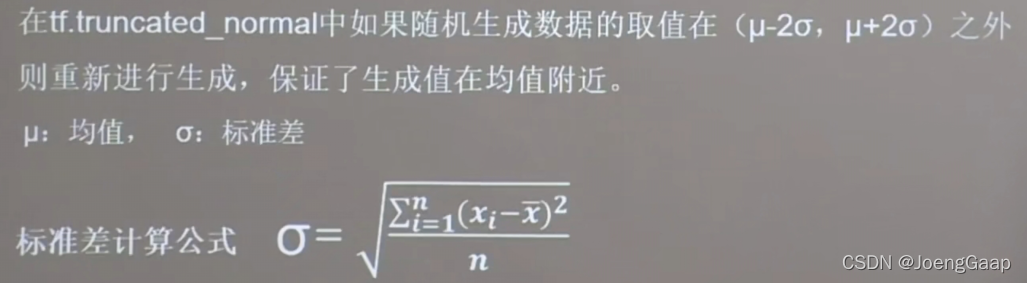
生成截断式正态分布的随机数
tf.random.truncated_normal(维度,mean=均值,stddev=标准差)
import tensorflow as tf
d=tf.random.normal([2,2],mean=0.5,stddev=1)
print(d)
e=tf.random.truncated_normal([2,2],mean=0.5,stddev=1)
print(e)
运行结果:
tf.Tensor(
[[1.5250179 1.2026441]
 [0.9217689 1.0258312]], shape=(2, 2), dtype=float32)
tf.Tensor(
[[ 1.465446    1.1151301 ]
 [ 0.14352742 -0.14995104]], shape=(2, 2), dtype=float32)
生成均匀分布随机数
tf.random.uniform(维度,minival=最小值,maxval=最大值)
import tensorflow as tf
f=tf.random.uniform([2,2],minval=0,maxval=1)
print(f)
运行结果:
tf.Tensor(
[[0.6806916  0.83334017]
 [0.29445708 0.3013816 ]], shape=(2, 2), dtype=float32)
常用函数
强制tensor转换为该数据类型
tf.cast(张量名,dtype=数据类型)
计算张量维度上元素的最小值
tf.reduce_min(张量名)
计算张量维度上元素的最大值
tf.reduce_max(张量名)
import tensorflow as tf
x1=tf.constant([1.,2.,3.],dtype=tf.float64)
print(x1)
x2=tf.cast(x1,tf.int32)
print(x2)
print(tf.reduce_min(x2),tf.reduce_max(x2))
运行结果:
tf.Tensor([1. 2. 3.], shape=(3,), dtype=float64)
tf.Tensor([1 2 3], shape=(3,), dtype=int32)
tf.Tensor(1, shape=(), dtype=int32) tf.Tensor(3, shape=(), dtype=int32)
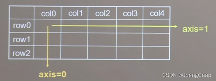
理解axis
在一个二维张量或者数组中,可以通过调整axis等于0或1控制执行维度。
axis=0代表跨行(经度,down),而axis=1表示跨列(纬度,across)
如果不指定axis,则所有元素参与计算
计算张量沿着指定维度的平均值
tf.reduce_mean(张量名,axis=操作轴)
计算张量沿着指定维度的和
tf.reduce_sum(张量名,axis=操作轴)
import tensorflow as tf
x=tf.constant([[1,2,3],[2,2,3]])
print(x)
print(tf.reduce_mean(x))
print(tf.reduce_sum(x,axis=1))
运行结果:
tf.Tensor(
[[1 2 3]
 [2 2 3]], shape=(2, 3), dtype=int32)
tf.Tensor(2, shape=(), dtype=int32)
tf.Tensor([6 7], shape=(2,), dtype=int32)
tf.Variable()
tf.Variable(初始值)将变量标记为“可训练”,被标记的变量会在反向传播中记录梯度信息。神经网络训练中,常用该函数标记待训练参数。
w=tf.Variable(tf.random.normal([2,2],mean=0,stddev=1))
Tensorflow中的数学运算
对应元素的四则运算:tf.add(张量1,张量2), tf.subtract(张量1,张量2), tf.multiply(张量1,张量2), tf.divide(张量1,张量2)
(只有相同维度的张量才可以做四则运算)
平方、次方与开方:tf.square(张量名), tf.pow(张量名,n次方数), tf.sqrt(张量名)
矩阵乘:tf.matmul(矩阵1,矩阵2)
import tensorflow as tf
a=tf.ones([3,3],dtype=tf.float32)
b=tf.fill([3,3],3.)
print(a)
print(b)
print(tf.add(a,b))
print(tf.subtract(a,b))
print(tf.multiply(a,b))
print(tf.divide(b,a))
print(tf.pow(b,3))
print(tf.square(b))
print(tf.sqrt(b))#张量数据类型要为浮点类型
print(tf.matmul(a,b))#注意两个矩阵的维度
运行结果:
tf.Tensor(
[[1. 1. 1.]
 [1. 1. 1.]
 [1. 1. 1.]], shape=(3, 3), dtype=float32)
tf.Tensor(
[[3. 3. 3.]
 [3. 3. 3.]
 [3. 3. 3.]], shape=(3, 3), dtype=float32)
tf.Tensor(
[[4. 4. 4.]
 [4. 4. 4.]
 [4. 4. 4.]], shape=(3, 3), dtype=float32)
tf.Tensor(
[[-2. -2. -2.]
 [-2. -2. -2.]
 [-2. -2. -2.]], shape=(3, 3), dtype=float32)
tf.Tensor(
[[3. 3. 3.]
 [3. 3. 3.]
 [3. 3. 3.]], shape=(3, 3), dtype=float32)
tf.Tensor(
[[3. 3. 3.]
 [3. 3. 3.]
 [3. 3. 3.]], shape=(3, 3), dtype=float32)
tf.Tensor(
[[27. 27. 27.]
 [27. 27. 27.]
 [27. 27. 27.]], shape=(3, 3), dtype=float32)
tf.Tensor(
[[9. 9. 9.]
 [9. 9. 9.]
 [9. 9. 9.]], shape=(3, 3), dtype=float32)
tf.Tensor(
[[1.7320508 1.7320508 1.7320508]
 [1.7320508 1.7320508 1.7320508]
 [1.7320508 1.7320508 1.7320508]], shape=(3, 3), dtype=float32)
tf.Tensor(
[[9. 9. 9.]
 [9. 9. 9.]
 [9. 9. 9.]], shape=(3, 3), dtype=float32)
切分传入张量的第一维度,生成输入特征/标签对,构建数据集
data=tf.data.Dataset.from_tensor_slices((输入特征,标签))
numpy和Tensor格式都可用该语句读入数据
import tensorflow as tf
features=tf.constant([12,23,10,17])
labels=tf.constant([0,1,1,0])
dataset=tf.data.Dataset.from_tensor_slices((features,labels))
print(dataset)
for element in dataset:
    print(element)
运行结果:
<TensorSliceDataset shapes: ((), ()), types: (tf.int32, tf.int32)>
(<tf.Tensor: shape=(), dtype=int32, numpy=12>, <tf.Tensor: shape=(), dtype=int32, numpy=0>)
(<tf.Tensor: shape=(), dtype=int32, numpy=23>, <tf.Tensor: shape=(), dtype=int32, numpy=1>)
(<tf.Tensor: shape=(), dtype=int32, numpy=10>, <tf.Tensor: shape=(), dtype=int32, numpy=1>)
(<tf.Tensor: shape=(), dtype=int32, numpy=17>, <tf.Tensor: shape=(), dtype=int32, numpy=0>)
tf.GradientTape()
with结构记录计算过程,gradient求出张量的梯度
with tf.GradientTape() as tape:
若干个计算过程
grad=tape.gradient(函数,对谁求导)
import tensorflow as tf
with tf.GradientTape() as tape:
    w=tf.Variable(tf.constant(3.0))
    loss=tf.pow(w,2)
grad=tape.gradient(loss,w)
print(grad)
运行结果:
tf.Tensor(6.0, shape=(), dtype=float32)
enumerate
enumerate(列表名)是python的内建函数,它可遍历每个元素(如列表、元组或字符串),组合为:索引 元素,常在for循环中使用。
import tensorflow as tf
seq=["one","two","three"]
for i,element in enumerate(seq):
    print(i,element)
运行结果:
0 one
1 two
2 three
独热编码(one-hot encoding)
在分类问题中,常用独热编码做标签,标记类别:1,0
tf.one_hot(待转换数据,depth=几分类)
import tensorflow as tf
classes=3
labels=tf.constant([1,0,2])
output=tf.one_hot(labels,classes)
print(output)
运行结果:
tf.Tensor(
[[0. 1. 0.]
 [1. 0. 0.]
 [0. 0. 1.]], shape=(3, 3), dtype=float32)
tf.nn.softmax
当n分类的n个输出(y0,y1,…,yn-1)通过softmax函数,便符合概率分布了

import tensorflow as tf
y=tf.constant([1.01,2.01,-0.66])
y_pro=tf.nn.softmax(y)
print(y_pro)
运行结果:
tf.Tensor([0.25598174 0.69583046 0.04818781], shape=(3,), dtype=float32)
assign_sub
赋值操作,更新参数的值并返回
调用assign_sub(w要自减的内容)前,先用tf.Variable定义变量w为可训练
import tensorflow as tf
w=tf.Variable(4)
w.assign_sub(1)
print(w)
运行结果:
<tf.Variable 'Variable:0' shape=() dtype=int32, numpy=3>
tf.argmax(张量名,axis=操作轴)
返回张量沿着指定维度最大值的索引
import tensorflow as tf
import numpy as np
test=np.array([[1,2,3],[2,3,4],[3,4,5]])
print(test)
print(tf.argmax(test,axis=0))
print(tf.argmax(test,axis=1))
运行结果:
[[1 2 3]
 [2 3 4]
 [3 4 5]]
tf.Tensor([2 2 2], shape=(3,), dtype=int64)
tf.Tensor([2 2 2], shape=(3,), dtype=int64)
鸢尾花数据集读入
from sklearn import datasets
from pandas import DataFrame
import pandas as pd

x_data = datasets.load_iris().data  # .data返回iris数据集所有输入特征
y_data = datasets.load_iris().target  # .target返回iris数据集所有标签
print("x_data from datasets: \n", x_data)
print("y_data from datasets: \n", y_data)

x_data = DataFrame(x_data, columns=['花萼长度', '花萼宽度', '花瓣长度', '花瓣宽度']) # 为表格增加行索引(左侧)和列标签(上方)
pd.set_option('display.unicode.east_asian_width', True)  # 设置列名对齐
print("x_data add index: \n", x_data)

x_data['类别'] = y_data  # 新加一列,列标签为‘类别’,数据为y_data
print("x_data add a column: \n", x_data)
运行结果:
x_data from datasets:
 [[5.1 3.5 1.4 0.2]
 [4.9 3.  1.4 0.2]
 [4.7 3.2 1.3 0.2]
 [4.6 3.1 1.5 0.2]
 [5.  3.6 1.4 0.2]
 [5.4 3.9 1.7 0.4]
 [4.6 3.4 1.4 0.3]
 [5.  3.4 1.5 0.2]
 [4.4 2.9 1.4 0.2]
 [4.9 3.1 1.5 0.1]
 [5.4 3.7 1.5 0.2]
 [4.8 3.4 1.6 0.2]
 [4.8 3.  1.4 0.1]
 [4.3 3.  1.1 0.1]
 [5.8 4.  1.2 0.2]
 [5.7 4.4 1.5 0.4]
 [5.4 3.9 1.3 0.4]
 [5.1 3.5 1.4 0.3]
 [5.7 3.8 1.7 0.3]
 [5.1 3.8 1.5 0.3]
 [5.4 3.4 1.7 0.2]
 [5.1 3.7 1.5 0.4]
 [4.6 3.6 1.  0.2]
 [5.1 3.3 1.7 0.5]
 [4.8 3.4 1.9 0.2]
 [5.  3.  1.6 0.2]
 [5.  3.4 1.6 0.4]
 [5.2 3.5 1.5 0.2]
 [5.2 3.4 1.4 0.2]
 [4.7 3.2 1.6 0.2]
 [4.8 3.1 1.6 0.2]
 [5.4 3.4 1.5 0.4]
 [5.2 4.1 1.5 0.1]
 [5.5 4.2 1.4 0.2]
 [4.9 3.1 1.5 0.2]
 [5.  3.2 1.2 0.2]
 [5.5 3.5 1.3 0.2]
 [4.9 3.6 1.4 0.1]
 [4.4 3.  1.3 0.2]
 [5.1 3.4 1.5 0.2]
 [5.  3.5 1.3 0.3]
 [4.5 2.3 1.3 0.3]
 [4.4 3.2 1.3 0.2]
 [5.  3.5 1.6 0.6]
 [5.1 3.8 1.9 0.4]
 [4.8 3.  1.4 0.3]
 [5.1 3.8 1.6 0.2]
 [4.6 3.2 1.4 0.2]
 [5.3 3.7 1.5 0.2]
 [5.  3.3 1.4 0.2]
 [7.  3.2 4.7 1.4]
 [6.4 3.2 4.5 1.5]
 [6.9 3.1 4.9 1.5]
 [5.5 2.3 4.  1.3]
 [6.5 2.8 4.6 1.5]
 [5.7 2.8 4.5 1.3]
 [6.3 3.3 4.7 1.6]
 [4.9 2.4 3.3 1. ]
 [6.6 2.9 4.6 1.3]
 [5.2 2.7 3.9 1.4]
 [5.  2.  3.5 1. ]
 [5.9 3.  4.2 1.5]
 [6.  2.2 4.  1. ]
 [6.1 2.9 4.7 1.4]
 [5.6 2.9 3.6 1.3]
 [6.7 3.1 4.4 1.4]
 [5.6 3.  4.5 1.5]
 [5.8 2.7 4.1 1. ]
 [6.2 2.2 4.5 1.5]
 [5.6 2.5 3.9 1.1]
 [5.9 3.2 4.8 1.8]
 [6.1 2.8 4.  1.3]
 [6.3 2.5 4.9 1.5]
 [6.1 2.8 4.7 1.2]
 [6.4 2.9 4.3 1.3]
 [6.6 3.  4.4 1.4]
 [6.8 2.8 4.8 1.4]
 [6.7 3.  5.  1.7]
 [6.  2.9 4.5 1.5]
 [5.7 2.6 3.5 1. ]
 [5.5 2.4 3.8 1.1]
 [5.5 2.4 3.7 1. ]
 [5.8 2.7 3.9 1.2]
 [6.  2.7 5.1 1.6]
 [5.4 3.  4.5 1.5]
 [6.  3.4 4.5 1.6]
 [6.7 3.1 4.7 1.5]
 [6.3 2.3 4.4 1.3]
 [5.6 3.  4.1 1.3]
 [5.5 2.5 4.  1.3]
 [5.5 2.6 4.4 1.2]
 [6.1 3.  4.6 1.4]
 [5.8 2.6 4.  1.2]
 [5.  2.3 3.3 1. ]
 [5.6 2.7 4.2 1.3]
 [5.7 3.  4.2 1.2]
 [5.7 2.9 4.2 1.3]
 [6.2 2.9 4.3 1.3]
 [5.1 2.5 3.  1.1]
 [5.7 2.8 4.1 1.3]
 [6.3 3.3 6.  2.5]
 [5.8 2.7 5.1 1.9]
 [7.1 3.  5.9 2.1]
 [6.3 2.9 5.6 1.8]
 [6.5 3.  5.8 2.2]
 [7.6 3.  6.6 2.1]
 [4.9 2.5 4.5 1.7]
 [7.3 2.9 6.3 1.8]
 [6.7 2.5 5.8 1.8]
 [7.2 3.6 6.1 2.5]
 [6.5 3.2 5.1 2. ]
 [6.4 2.7 5.3 1.9]
 [6.8 3.  5.5 2.1]
 [5.7 2.5 5.  2. ]
 [5.8 2.8 5.1 2.4]
 [6.4 3.2 5.3 2.3]
 [6.5 3.  5.5 1.8]
 [7.7 3.8 6.7 2.2]
 [7.7 2.6 6.9 2.3]
 [6.  2.2 5.  1.5]
 [6.9 3.2 5.7 2.3]
 [5.6 2.8 4.9 2. ]
 [7.7 2.8 6.7 2. ]
 [6.3 2.7 4.9 1.8]
 [6.7 3.3 5.7 2.1]
 [7.2 3.2 6.  1.8]
 [6.2 2.8 4.8 1.8]
 [6.1 3.  4.9 1.8]
 [6.4 2.8 5.6 2.1]
 [7.2 3.  5.8 1.6]
 [7.4 2.8 6.1 1.9]
 [7.9 3.8 6.4 2. ]
 [6.4 2.8 5.6 2.2]
 [6.3 2.8 5.1 1.5]
 [6.1 2.6 5.6 1.4]
 [7.7 3.  6.1 2.3]
 [6.3 3.4 5.6 2.4]
 [6.4 3.1 5.5 1.8]
 [6.  3.  4.8 1.8]
 [6.9 3.1 5.4 2.1]
 [6.7 3.1 5.6 2.4]
 [6.9 3.1 5.1 2.3]
 [5.8 2.7 5.1 1.9]
 [6.8 3.2 5.9 2.3]
 [6.7 3.3 5.7 2.5]
 [6.7 3.  5.2 2.3]
 [6.3 2.5 5.  1.9]
 [6.5 3.  5.2 2. ]
 [6.2 3.4 5.4 2.3]
 [5.9 3.  5.1 1.8]]
y_data from datasets:
 [0 0 0 0 0 0 0 0 0 0 0 0 0 0 0 0 0 0 0 0 0 0 0 0 0 0 0 0 0 0 0 0 0 0 0 0 0
 0 0 0 0 0 0 0 0 0 0 0 0 0 1 1 1 1 1 1 1 1 1 1 1 1 1 1 1 1 1 1 1 1 1 1 1 1
 1 1 1 1 1 1 1 1 1 1 1 1 1 1 1 1 1 1 1 1 1 1 1 1 1 1 2 2 2 2 2 2 2 2 2 2 2
 2 2 2 2 2 2 2 2 2 2 2 2 2 2 2 2 2 2 2 2 2 2 2 2 2 2 2 2 2 2 2 2 2 2 2 2 2
 2 2]
x_data add index:
      花萼长度  花萼宽度  花瓣长度  花瓣宽度
0         5.1       3.5       1.4       0.2
1         4.9       3.0       1.4       0.2
2         4.7       3.2       1.3       0.2
3         4.6       3.1       1.5       0.2
4         5.0       3.6       1.4       0.2
5         5.4       3.9       1.7       0.4
6         4.6       3.4       1.4       0.3
7         5.0       3.4       1.5       0.2
8         4.4       2.9       1.4       0.2
9         4.9       3.1       1.5       0.1
10        5.4       3.7       1.5       0.2
11        4.8       3.4       1.6       0.2
12        4.8       3.0       1.4       0.1
13        4.3       3.0       1.1       0.1
14        5.8       4.0       1.2       0.2
15        5.7       4.4       1.5       0.4
16        5.4       3.9       1.3       0.4
17        5.1       3.5       1.4       0.3
18        5.7       3.8       1.7       0.3
19        5.1       3.8       1.5       0.3
20        5.4       3.4       1.7       0.2
21        5.1       3.7       1.5       0.4
22        4.6       3.6       1.0       0.2
23        5.1       3.3       1.7       0.5
24        4.8       3.4       1.9       0.2
25        5.0       3.0       1.6       0.2
26        5.0       3.4       1.6       0.4
27        5.2       3.5       1.5       0.2
28        5.2       3.4       1.4       0.2
29        4.7       3.2       1.6       0.2
..        ...       ...       ...       ...
120       6.9       3.2       5.7       2.3
121       5.6       2.8       4.9       2.0
122       7.7       2.8       6.7       2.0
123       6.3       2.7       4.9       1.8
124       6.7       3.3       5.7       2.1
125       7.2       3.2       6.0       1.8
126       6.2       2.8       4.8       1.8
127       6.1       3.0       4.9       1.8
128       6.4       2.8       5.6       2.1
129       7.2       3.0       5.8       1.6
130       7.4       2.8       6.1       1.9
131       7.9       3.8       6.4       2.0
132       6.4       2.8       5.6       2.2
133       6.3       2.8       5.1       1.5
134       6.1       2.6       5.6       1.4
135       7.7       3.0       6.1       2.3
136       6.3       3.4       5.6       2.4
137       6.4       3.1       5.5       1.8
138       6.0       3.0       4.8       1.8
139       6.9       3.1       5.4       2.1
140       6.7       3.1       5.6       2.4
141       6.9       3.1       5.1       2.3
142       5.8       2.7       5.1       1.9
143       6.8       3.2       5.9       2.3
144       6.7       3.3       5.7       2.5
145       6.7       3.0       5.2       2.3
146       6.3       2.5       5.0       1.9
147       6.5       3.0       5.2       2.0
148       6.2       3.4       5.4       2.3
149       5.9       3.0       5.1       1.8

[150 rows x 4 columns]
x_data add a column:
      花萼长度  花萼宽度  花瓣长度  花瓣宽度  类别
0         5.1       3.5       1.4       0.2     0
1         4.9       3.0       1.4       0.2     0
2         4.7       3.2       1.3       0.2     0
3         4.6       3.1       1.5       0.2     0
4         5.0       3.6       1.4       0.2     0
5         5.4       3.9       1.7       0.4     0
6         4.6       3.4       1.4       0.3     0
7         5.0       3.4       1.5       0.2     0
8         4.4       2.9       1.4       0.2     0
9         4.9       3.1       1.5       0.1     0
10        5.4       3.7       1.5       0.2     0
11        4.8       3.4       1.6       0.2     0
12        4.8       3.0       1.4       0.1     0
13        4.3       3.0       1.1       0.1     0
14        5.8       4.0       1.2       0.2     0
15        5.7       4.4       1.5       0.4     0
16        5.4       3.9       1.3       0.4     0
17        5.1       3.5       1.4       0.3     0
18        5.7       3.8       1.7       0.3     0
19        5.1       3.8       1.5       0.3     0
20        5.4       3.4       1.7       0.2     0
21        5.1       3.7       1.5       0.4     0
22        4.6       3.6       1.0       0.2     0
23        5.1       3.3       1.7       0.5     0
24        4.8       3.4       1.9       0.2     0
25        5.0       3.0       1.6       0.2     0
26        5.0       3.4       1.6       0.4     0
27        5.2       3.5       1.5       0.2     0
28        5.2       3.4       1.4       0.2     0
29        4.7       3.2       1.6       0.2     0
..        ...       ...       ...       ...   ...
120       6.9       3.2       5.7       2.3     2
121       5.6       2.8       4.9       2.0     2
122       7.7       2.8       6.7       2.0     2
123       6.3       2.7       4.9       1.8     2
124       6.7       3.3       5.7       2.1     2
125       7.2       3.2       6.0       1.8     2
126       6.2       2.8       4.8       1.8     2
127       6.1       3.0       4.9       1.8     2
128       6.4       2.8       5.6       2.1     2
129       7.2       3.0       5.8       1.6     2
130       7.4       2.8       6.1       1.9     2
131       7.9       3.8       6.4       2.0     2
132       6.4       2.8       5.6       2.2     2
133       6.3       2.8       5.1       1.5     2
134       6.1       2.6       5.6       1.4     2
135       7.7       3.0       6.1       2.3     2
136       6.3       3.4       5.6       2.4     2
137       6.4       3.1       5.5       1.8     2
138       6.0       3.0       4.8       1.8     2
139       6.9       3.1       5.4       2.1     2
140       6.7       3.1       5.6       2.4     2
141       6.9       3.1       5.1       2.3     2
142       5.8       2.7       5.1       1.9     2
143       6.8       3.2       5.9       2.3     2
144       6.7       3.3       5.7       2.5     2
145       6.7       3.0       5.2       2.3     2
146       6.3       2.5       5.0       1.9     2
147       6.5       3.0       5.2       2.0     2
148       6.2       3.4       5.4       2.3     2
149       5.9       3.0       5.1       1.8     2

[150 rows x 5 columns]
神经网络实现鸢尾花分类
准备数据
- 数据集读入
- 数据集乱序
- 生成训练集和测试集
- 配成(输入特征,标签)对,每次读入一小撮(batch)
搭建网络
定义神经网络中所有可训练参数
参数优化
嵌套循环迭代,with结构更新参数,显示当前loss
测试效果
计算当前参数前向传播后的准确率,显示当前acc
acc/loss可视化
# -*- coding: UTF-8 -*-
# 利用鸢尾花数据集,实现前向传播、反向传播,可视化loss曲线

# 导入所需模块
import tensorflow as tf
from sklearn import datasets
from matplotlib import pyplot as plt
import numpy as np

# 导入数据,分别为输入特征和标签
x_data = datasets.load_iris().data
y_data = datasets.load_iris().target

# 随机打乱数据(因为原始数据是顺序的,顺序不打乱会影响准确率)
# seed: 随机数种子,是一个整数,当设置之后,每次生成的随机数都一样(为方便教学,以保每位同学结果一致)
np.random.seed(116)  # 使用相同的seed,保证输入特征和标签一一对应
np.random.shuffle(x_data)
np.random.seed(116)
np.random.shuffle(y_data)
tf.random.set_seed(116)

# 将打乱后的数据集分割为训练集和测试集,训练集为前120行,测试集为后30行
x_train = x_data[:-30]
y_train = y_data[:-30]
x_test = x_data[-30:]
y_test = y_data[-30:]

# 转换x的数据类型,否则后面矩阵相乘时会因数据类型不一致报错
x_train = tf.cast(x_train, tf.float32)
x_test = tf.cast(x_test, tf.float32)

# from_tensor_slices函数使输入特征和标签值一一对应。(把数据集分批次,每个批次batch组数据)
train_db = tf.data.Dataset.from_tensor_slices((x_train, y_train)).batch(32)
test_db = tf.data.Dataset.from_tensor_slices((x_test, y_test)).batch(32)

# 生成神经网络的参数,4个输入特征故,输入层为4个输入节点;因为3分类,故输出层为3个神经元
# 用tf.Variable()标记参数可训练
# 使用seed使每次生成的随机数相同(方便教学,使大家结果都一致,在现实使用时不写seed)
w1 = tf.Variable(tf.random.truncated_normal([4, 3], stddev=0.1, seed=1))
b1 = tf.Variable(tf.random.truncated_normal([3], stddev=0.1, seed=1))

lr = 0.1  # 学习率为0.1
train_loss_results = []  # 将每轮的loss记录在此列表中,为后续画loss曲线提供数据
test_acc = []  # 将每轮的acc记录在此列表中,为后续画acc曲线提供数据
epoch = 500  # 循环500轮
loss_all = 0  # 每轮分4个step,loss_all记录四个step生成的4个loss的和

# 训练部分
for epoch in range(epoch):  #数据集级别的循环,每个epoch循环一次数据集
    for step, (x_train, y_train) in enumerate(train_db):  #batch级别的循环 ,每个step循环一个batch
        with tf.GradientTape() as tape:  # with结构记录梯度信息
            y = tf.matmul(x_train, w1) + b1  # 神经网络乘加运算
            y = tf.nn.softmax(y)  # 使输出y符合概率分布(此操作后与独热码同量级,可相减求loss)
            y_ = tf.one_hot(y_train, depth=3)  # 将标签值转换为独热码格式,方便计算loss和accuracy
            loss = tf.reduce_mean(tf.square(y_ - y))  # 采用均方误差损失函数mse = mean(sum(y-out)^2)
            loss_all += loss.numpy()  # 将每个step计算出的loss累加,为后续求loss平均值提供数据,这样计算的loss更准确
        # 计算loss对各个参数的梯度
        grads = tape.gradient(loss, [w1, b1])

        # 实现梯度更新 w1 = w1 - lr * w1_grad    b = b - lr * b_grad
        w1.assign_sub(lr * grads[0])  # 参数w1自更新
        b1.assign_sub(lr * grads[1])  # 参数b自更新

    # 每个epoch,打印loss信息
    print("Epoch {}, loss: {}".format(epoch, loss_all/4))
    train_loss_results.append(loss_all / 4)  # 将4个step的loss求平均记录在此变量中
    loss_all = 0  # loss_all归零,为记录下一个epoch的loss做准备

    # 测试部分
    # total_correct为预测对的样本个数, total_number为测试的总样本数,将这两个变量都初始化为0
    total_correct, total_number = 0, 0
    for x_test, y_test in test_db:
        # 使用更新后的参数进行预测
        y = tf.matmul(x_test, w1) + b1
        y = tf.nn.softmax(y)
        pred = tf.argmax(y, axis=1)  # 返回y中最大值的索引,即预测的分类
        # 将pred转换为y_test的数据类型
        pred = tf.cast(pred, dtype=y_test.dtype)
        # 若分类正确,则correct=1,否则为0,将bool型的结果转换为int型
        correct = tf.cast(tf.equal(pred, y_test), dtype=tf.int32)
        # 将每个batch的correct数加起来
        correct = tf.reduce_sum(correct)
        # 将所有batch中的correct数加起来
        total_correct += int(correct)
        # total_number为测试的总样本数,也就是x_test的行数,shape[0]返回变量的行数
        total_number += x_test.shape[0]
    # 总的准确率等于total_correct/total_number
    acc = total_correct / total_number
    test_acc.append(acc)
    print("Test_acc:", acc)
    print("--------------------------")

# 绘制 loss 曲线
plt.title('Loss Function Curve')  # 图片标题
plt.xlabel('Epoch')  # x轴变量名称
plt.ylabel('Loss')  # y轴变量名称
plt.plot(train_loss_results, label="$Loss$")  # 逐点画出trian_loss_results值并连线,连线图标是Loss
plt.legend()  # 画出曲线图标
plt.show()  # 画出图像

# 绘制 Accuracy 曲线
plt.title('Acc Curve')  # 图片标题
plt.xlabel('Epoch')  # x轴变量名称
plt.ylabel('Acc')  # y轴变量名称
plt.plot(test_acc, label="$Accuracy$")  # 逐点画出test_acc值并连线,连线图标是Accuracy
plt.legend()
plt.show()


 1110
1110


 被折叠的 条评论
为什么被折叠?
被折叠的 条评论
为什么被折叠?
 到【灌水乐园】发言


