


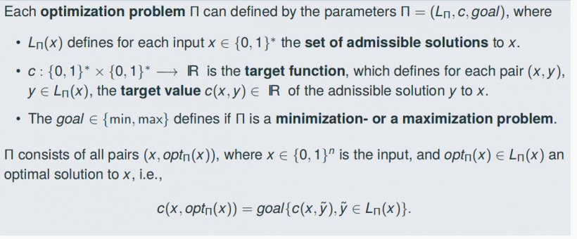
1. Introduction: Problems, Algorithms, Computations
1.1Computational problems
Computational problems Π are relations Π ⊆ X × Y between a set X of valid inputs, and a set Y of valid outputs.
(x, y) ∈ Π means: y is a solution of x w.r.t. Π.
1.2 Input and Input length
1.3 Algorithms
Algorithms A are instructions for a device to execute a well defined sequence of computational steps in dependence of the stored input data x (one elementary operation per step)
This sequence is called computation of A on x and can be finite or infinite.
1.4 Cost measures for computations
time consumption timeA(x) = the sum of the time costs of the computational steps of the computation
The execution of one elementary operation costs one time unit => make time platform independent
space consumption spaceA(x) = the number of storage units used during
the computation of A on
1.5 Time Behaviour of Algorithms
Worst Case Running Time
Best Case RT
Average Case RT
1.6 Design and Analysis of Algorithms(Roadmap)
Design -> Proof of Correctness -> Analysis of the Running Time
1.7 Asymptotic Growth Order of Function, O-Notation
neglect multiplicative constants and additive low order terms
- f(n) = O(g(n)): f grows asymptotically not faster than g => I can choose a C ∈ R>0, such that from a certain point on f(n) is never greater than C · g(n).
- f(n) = Ω(g(n)): f grows asymptotically not slower than g => I can choose a C ∈ R>0, such that from a certain point on f(n) is never smaller than C · g(n).
- f(n) = Θ(g(n)): f and g have the same asymptotic growth order
- f(n) = o(g(n)): f grows asymptotically strictly slower than g = > No matter how I choose C ∈ R>0, from a certain point on f(n) is always smaller than C · g(n).
- f(n) = ω(g(n)): f grows asymptotically strictly faster than g => No matter how I choose C ∈ R>0, from a certain point on f(n) is always greater than C · g(n).
1.8 Efficiently solvable problems
A problem Π is considered to be efficiently solvable, if there is a polynomial time
algorithm A for Π.
Exponential time is not efficient in practice.
1.9 PTIME
PTIME denotes the set of all problems, which have a polynomial time algorithm in some reasonable model of computation (i.e., in all reasonable models of computation)
2. Shortest Path Problems
Shortest Paths: A path p from a node u to a node v is called shortest path from u
to v if for all paths p0 from u to v it holds w(p0 ) ≥ w§.
2.1 Types
- Single Pair Shortest Path
- Single Source Shortest Path
- All Pairs Shortest Path
2.2 Walks, Paths, Cycles
- Walks: A sequence of consecutive edges
p = ((v0, v1),(v1, v2), · · · ,(vk−2, vk−1),(vk−1, vk ))
is called walk in G from v0 to vk of length k. - Paths: The walk p is called path if vi is not equals to vj for all 1 ≤ i < j ≤ k.
- Cycles: The path p is called cycle if v0 = vk
2.3 Distances in Weighted Graphs G = (V,E, w)
Distance δG(u, v) from node u to node v
- δG(u, v) = ∞: v is not reachable from u in G
- δG(u, v) = −∞: there is a walk from u to v containing a cycle K of negative weight
- δG(u, v) = w§: v is reachable from u in G and no walk from u to v contains a negative cycle and p denotes a shortest path from u to v
2.4 Properties of Shortest Paths
- Let G = (V, E, w) be a weighted graph, and let s, u, v ∈ V. If −∞ < δG(u, v) < ∞ then there is a shortest walk p from u to v which is a path and which has at most |V| − 1 edges.
Proof: Then each cycle has non negative weight and can be removed + Each path (without cycles) in G has at most |V| − 1 edges. - Monotonicity
the subpath of a shortest path is also a shortest path. - Triangle Inequality
δG(s, v) ≤ δG(s, u) + w(u, v)
proof: consider three possibilities- u is not reachable from s, i.e., u.d = ∞.
- u is reachable from s, but there is no shortest path from s to v going through u
- u is reachable from s and there is a shortest path from s to v going through u
2.5 Basic Operations Initialize and Relax
Initialize(G, s):
For all v ∈ V
	do v.d ← ∞ // set a path from s to v is infinite
		v.π ← NIL
s.d ← 0 // set the distance of s to s is 0
Running time O(|V|).

Relax(u, v, w):
If v.d > u.d + w(u, v)
	// Relax edge (u, v)
	then v.d ← u.d + w(u, v)
		v.π ← u // set new previous sector( s->u->v)
Running time O(1)
2.6 Subgraph Gπ = (Vπ, Eπ)
Vπ = {v ∈ V, v.d < ∞}
Eπ = {(v.π, v), v.π /=(not equals to) NIL}
Suppose that no negative cycle is reachable from s.
Then Gπ is always a tree with root s, and
For each v ∈ Vπ it holds that v.d = δGπ (s, v) ≥ δG(s, v).
I.e., v.d denotes the length of the path from s to v in the tree Gπ.
(Proof: Gπ is a disjoint union of one tree with root s and some cycles -> Gπ is acyclic
Any cycle K = (v1, · · · , vk, v1) in Gπ which is reachable from s in G has negative weight)
2.7 Bellman-Ford Algorithm
BellmanFord(G, w, s):
Initialize(G, s)
For i ← 1 to |V| − 1
	do for all (u, v) ∈ E
		do Relax(u, v, w)
For all (u, v) ∈ E
	do if v.d > u.d + w(u, v)
		then return false, STOP
return true

Running time O(|V||E|)
BellmanFord(G, w, s) outputs true if and only if no negative cycle is reachable from s. In this case, the output Gπ is a shortest path tree with root s which contains all nodes v which are reachable from s.
(Proof: induction over i that for all i, 1 ≤ i ≤ k, it holds (vi).d = δG(s, vi) after round i.
Case i = 1, …
Case i > 1,…)
Suppose there is a function f : V −→ R ∪ {∞} fulfilling f(v) ≤ f(u) + w(u, v) for all edges (u, v) ∈ E, where f(v) /= ∞ for all nodes v reachable from s. Then all cycles K = (v1, · · · , vk , v1) which are reachable from s have non negative weight.
(Proof)
3. Formalizing Optimization Problems by Linear Programs and Integer Linear Programs
3.1 Linear Programs
linear function: f(λ · x) = λ · f(x) and f(x + y) = f(x) + f(y).
linear halfspace/ linear restriction
hyperplane

linear polyhedron: A subset Π of IR^n, formed by the intersection of a finite number of linear halfspaces,
Linear Program (or a Linear Programming Instance, for short, LP-instance):
I = (n, c, Π) is defined by
- a dimension n ∈ N+
- a linear target function c: R^n → R
- a linear polyhedron Π ⊆ R^n determining the set of admissible solutions.
To solve the LP-instance I = (n, c, Π) = determine some optimum x_opt ∈ Π
such that c(x_opt) = min{c(x); x ∈ Π}.
3.2 Integer Linear Program
An Integer Linear Program is defined by an LP-Instance I = (n, c, Π) and the additional
restriction that solutions have to have integral components.
- The Single-Pair Shortest Path problem as Integer Linear Program
- The Single Source Shortest Path problem as LP-problem
4. Solving Linear Programs
4.1 Convex Sets & inner point & extremal point
For x, y ∈ IR^n, let Line(x, y) = {x + λ(y − x), λ ∈ [0, 1]} be the line connecting x and y
A subset X ⊆ IR^n is called convex, if for all x, y ∈ X it holds that Line(x, y) ⊆ X.
when x ∈ X a point in X
- x is called inner point, if there are points y, z ∈ X \ {x} with x ∈ Line(y, z).
- x ∈ X is called extremal point if it is not an inner point.
Euclidean distance
Each linear polyhedron Π is convex
4.2 Optimal points
global minimum & global maximum
local minimum & local maximum
Let X ⊆ IR^n be a convex set and let c be a linear target function.
(1) Each local optimum of c on X is a global optimum of c on X.
(2) If X has a global optimum w.r.t c then it is also taken in an extremal point of X.
(Proof 1&2)
4.3 Characterizing Extremal Points of Linear Programs
linear restrictions

A subset of restrictions {Ri, i ∈ S}, S ⊆ {1, · · ·, m}, is called to be linearly independent, if the set of the corresponding rows {(ai,1, · · ·, ai,n); i ∈ S} of A is linearly independent,
i.e., they form an |S| × n-submatrix of A with rank |S|.
A point x ∈ Π is an extremal point of the linear polyhedron if and only if x satisfies a subset S of |S| = n linearly independent restrictions with equality
4.4 Exhaustive Search Algorithm

4.5 The Simplex Method, Basics
4.5.1 LP-instance in normal form
An LP-instance in normal form I = (n, m, c, z, A, b) has the form
max{c(x) − z; A ◦ x ≤ b, x ≥ 0 }
- n: dimension
- m: number of linear restrictions
- m + n: number of restrictions
- vector c = (c1, · · · , cn): target function c(x)
- A: coeficient matrix
- b: restriction vector
- z: a constant(could be omitted, but which plays a role in the Simplex method)
The underlying linear polyhedron is X(I) = {x; A ◦ x ≤ b, x ≥ 0 }.
4.5.2 Slacking Extensions

以下为个人理解,不对的麻烦大佬们指教!
slacking extensions中各项代表什么?
前n项是点坐标,后m项是将点分别带入m个约束方程再转化得到的项
为什么slacking extensions中各项不能为负值?
首先前n项d(d1, …, dn)应该满足xi ≥ 0的约束条件,其次后m项是由约束方程转化而来,为保证A ◦ x ≤ b即b - A ◦ x ≥ 0。因此slacking extensions中所有项必须都大于等于0。
为什么在slacking extensions中有n个项为0时,d为极值点?
若一个点为极值点,则该点是n条约束方程的交点,即该点必须满足至少n个约束方程,当slacking extensions中某项为0时,即代表该点满足约束方程(前n项为0意味着点在坐标轴上,即满足xi=0,后n项为0意味着点在约束方程线上,即满足b - A ◦ x = 0)
4.5.3 Basic Points
Let d = (d1, · · · , dn+m) ∈ IR^(n+m) denote the slacking extension of a point (d1, · · · , dn). Point d is called a basic point, if there is a set N ⊂ {x1, · · · , xn+m} of n linearly independent variables such that dk = 0 for all xk ∈ N.
In this case, N is called the set of non-basic variables of the basic point d and
B = {x1, · · · , xn+m} \ N is called the set of basic variables of d.
4.5.4 Admissible basic point
A basic point d is called admissible basic point if dk ≥ 0 for all k, 1 ≤ k ≤ n + m
4.5.5 Canonical basic point
The basic point (0 vector, b) = (0, 0, · · · , 0, b1, · · · , bm) is called the canonical basic point. It is admissible iff b ≥ 0 vector.(原点位置)
4.5.6 Slacking Normal Form of a Normal Form Instance I=(m,n,c,A,b)

The slacking variables xn+i measures the slacking distance of the restrictions Axi from the restriction bound bi.
The point d ∈ IR^n is a valid solution of I iff the slacking extension of d is a valid solution of SNF(I)
4.5.7 The Simplex Tableaux

4.6 The Simplex Method for non-negative restriction vectors
4.6.1 Direction Dq
Let I = (n, m, c, A, b) an normal form instance. Fact: If b ≥ 0 vector then (0 vector, b) is an admissible basic point.
Directions starting from (vector 0, b)
The point (vector 0, b) is left by n lines D1, · · · , Dn, called directions.
4.6.2 Improving and Bounded
For all q, 1 ≤ q ≤ n, direction Dq is defined by increasing component q.
Dq = {dq(λ), λ ≥ 0}
where dq(λ) = (0, · · · , 0, λ, 0 · · · , 0, b1 − λ · a1,q, · · · , bm − λ · am,q).
where λ stands at position q.
- Direction Dq is called bounded if there is some bound λ0 ≥ 0 such that dq(λ) is admissible if and only if 0 ≤ λ ≤ λ0
- A direction Dq is called improving if the target function strictly increases on Dq with increasing λ.(若目标函数q变量前的系数为正数,则improving)
Suppose that (vector 0, b) is an admissible basic point.
(i) A direction Dj, 1 ≤ j ≤ n, is improving if and only if cj > 0.
(ii) If cj ≤ 0 for all j, 1 ≤ j ≤ n, then (vector 0, b) is optimal.(若最终的目标方程中没有正的系数,说明任意方向都无法再improving,此时为optimal状态)
(Proof)
Bounded and Unbounded Directions
Suppose that (vector 0, b) is an admissible basic point and fix some j, 1 ≤ j ≤ n.
(i) Direction Dj is bounded 等价于 there is some i, 1 ≤ i ≤ m, such that ai,j > 0.(根据bounded定义要使bi − λ · ai,j ≥ 0且0 ≤ λ ≤ λ0,ai,j 必须大于0,否则λ可以为任意值,不存在临界值λ0)
(ii) In this case dj(λ) ∈ X(I) 等价于 0 ≤ λ ≤ min{ bi/ai,j ; 1 ≤ i ≤ m, ai,j > 0}(该点在bounded内)
Dj is an improving unbounded direction等价于cj > 0, and, for all i, 1 ≤ i ≤ m, ai,j ≤ 0. In this case, opt(I) = limλ→∞ cj · λ = ∞
4.6.3 Pivot Position
 Suppose that (vector 0, b) is not optimal, and that all improving directions starting at (vector 0, b) are bounded. Then there is a Pivot position (p, q), and: The point y = dq( bp/ap,q ) is an admissible basic point with c(y) > c((vector 0, b)). (像improving方向q移动到临界值bp/ap,q,此时是一个admissible basic point,且带入目标方程后更大)
(Proof)
4.7 Scheme of the Simplex Method


SimplexSearch(T) (* T admissible Simplex Tableaux *):
1 Repeat if T not optimal
2 		then if T not unbounded
3 				then choose Pivot Position (p, q)
4 						T ← Pivotp,q(T)
5 until T optimal or unbounded
6 Output T

4.8 Degenerate Simplex
Degenerate Pivot steps: If T’= Pivotp,q(T) and tp,0 = 0 then x(T) = x(T’)
Degenerate Pivot can occur in admissible basic points with more than n zeros.
Making a degenerate Pivot step means staying in the same basic point but changing to another set of n non-basic variables
4.9 Terminate
- If SimplexSearch(T) performs only non degenerate Pivot steps then it always
terminates - If it performs also degenerate Pivot steps then it may not terminate, if the heuristic of choosing the next Pivot position is badly designed.
- By an appropriate control structure, it should be ensured that SimplexSearch(T)
never visits tableaux which are defined w.r.t. the same set of nonbasic variables.
4.10 The Simplex Method for Restriction Vectors with Negative Components


4.11 Running time of the Simplex Method
Worst Case Running Time: exponential in n and m
Average running time : polynomial
5 The Maximum Flow Problem
5.1 Maximum flow problem
The Maximum Flow Problem refers to a system in which a material courses from
a source to a sink, where the source is the place where the material is produced and the sink is the place where the material is consumed.
5.2 Flow networks G(V,E,c)
a directed graph G=(V,E), and is defined as follows:
- There is a distinguished nonempty set S*⊆V called the set of sources.
- There is another non-empty distinguished set T⊆V, S∩T*= ∅, called the set of
sinks - There is a capacity function c : E → IR , where c(e) > 0 for all e ∈ E.
(For u, v ∈ V let a capacity value c(u, v) = 0 be equivalent to (u, v) do not belong to E)
5.3 Flows on Flow Networks


5.4 The Maximum Flow Problem
- Input: G = (V, E, c) flow network with S*, T* ⊆ V
- Output: A flow on G with maximal value
5.5 Restricted flow networks
A flow network G = (V, E, c) is called restricted if it contains only one source s ∈ V and one sink t ∈ V, where indegG(s) = outdegG(t) = 0.
Moreover, G does not contain pairs (u, v), (v, u) of antiparallel edges
5.6 Efficient Simulation of General Flow Networks by Restricted Ones
Let G = (V, E, c) be a general flow network with set of sources S* and set of sinks T*.
Then there is a restricted network G’ = (V’, E’, c’) with |V’| ≤ |V| + |E|/2 + 2, such that each flow on G corresponds to a flow on G’ with the same value, and vice versa
- add a new source s
- add a new sink t
- for all pairs (v,w),(w,v) of antiparallel in E => add a new vertex y and replace edge (w,v) by two new edges (w,y), (y,v) with c’(w,y)=c’(y,v)=c’(w,v)
Claim: Each flow f on G corresponds to a flow f’ on G’ (and vice versa) with |f| = |f’|
Maximum flow instances G = (V, E, c) can be formulated as LP-instances
5.7 Ford-Fulkerson Method: Residual Networks
 Ef consists of forward edges (u, v), for which (u, v) ∈ E and f(u, v) < c(u, v), and backward edges (v, u), for which (u, v) ∈ E and f(u, v) > 0
5.7.1 Basic on Residual Networks
The capacity cf(u, v) of a forward edge (u, v) ∈ Ef indicates the maximal value by which the flow through (u, v) ∈ E on G can be increased.
The capacity cf(v, u) of a backward edge (v, u) ∈ Ef indicates the maximal value by which the flow through the corresponding edge (u, v) ∈ E can be decreased.
5.7.2 Special Flow on Gf: Augmenting Paths
Each directed path p from s to t in Gf is called an augmenting path with respect to G and f. and we denote by cf(p)= min{cf(e), e ∈ p} the minimal capacity of p.
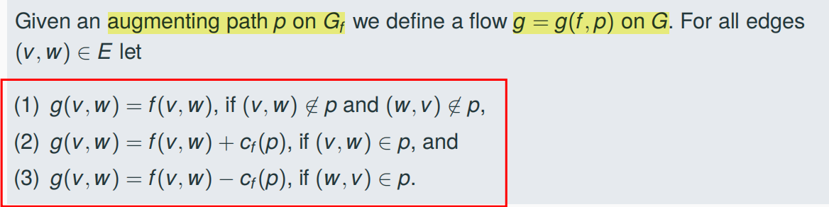
The mapping g = g(f, fp) defines a flow on G and it holds |g| = |f| + cf(p)
5.7.3 Cuts in G

Let f be a flow on G and (S, T) be a cut. Then |f| = f(S,T)
For all flows f on G = (V, E, c) and cuts (S, T) of V it holds |f| ≤ c(S, T)
Let G = (V, E, c) be a flow network and f a flow on G. Conditions (1) to (3) are equivalent
(1) The flow f is maximal.
(2) There is no path from s to t in Gf .
(3) There is a cut (S, T) such that |f| = c(S, T).
5.7.4 Ford-Fulkerson Method
Input: A Flow Network G = (V, E, s, t, c)
Output: A maximal flow f : E → IR .

Let f be the constant-0 flow on G
Repeat
		Fix a path p from s to t in Gf
		f ← g(f, fp)
until t is not reachable from s in Gf
Output f
5.8 Edmonds-Karp Algorithm
If in each iteration a shortest augmenting path is chosen, then Ford-Fulkerson terminates after O(|V|·|E|) iterations. This corresponds to the Edmonds-Karp Algorithm
Given a flow f on G = (V, E, c) and nodes u, v ∈ V, we denote by δf(u, v) the distance of v from u in Gf, i.e. the length (=number of edges) of a shortest path from u to v in Gf .
Now suppose f is a flow on G = (V, E, c) and flow f’ is obtained from f by one iteration of Ford-Fulkerson, where the corresponding augmenting path is a shortest path from s to t.
For all v ∈ V it holds that δf(s, v) ≤ δf’(s, v).
5.9 Correctness Theorem
Given a flow f on G = (V, E, c) and an augmenting path p in Gf. An edge e = (u, v) from p is called critical, if it has minimal capacity in p, i.e., cf(e) = cf§
During the execution of the Edmonds-Karp Algorithm on a flow network G = (V, E, c), each edge e ∈ E can become critical at most |V|/2 times
The Karp-Edmonds Algorithm stops after at most |E| ·(|V|/2) iterations. Thus the running time is O(|V|·|E|/2)
6. Matchings in Undirected Graphs
6.1 The Maximum Matching Problem
Input: An undirected graph G = (U, E).
Output: A maximal matching in G, i.e., a matching M ⊆ E in G with maximal number of edges.

6.2 Characterizing Maximum Matchings by Augmenting Paths
A node v ∈ V is called M-exposed if no edge of M contains v.
A simple path p in G is called M-augmenting, if its endpoints are M-exposed and, if p has more than one edge, it contains alternatingly edges which are not in M and edges which are in M.
A matching M ⊆ E is maximal if and only if there is no M-augmenting path
6.3 Maximal Matchings in Bipartite Graphs
An undirected graph G = (U, E) is called bipartite, if there is a partition U = V ∪ W of the node set into two disjoint subsets such that for all edges e = {v, w} ∈ E it holds that v ∈ V and w ∈ W.
6.4 Solving the Maximal Matching Problem for Bipartite Graphs
Step1: Transform the bipartite input graph G = (V, W, E) into a flow network G’ = (V’, E’, c)
Step2: Compute a maximum flow on G’ with Ford-Fulkerson
A maximal matching in a bipartite graph G = (V, W, E) can be computed in
time O(min{|V|, |W|} · |E|) by applying the Ford-Fulkerson Method.
6.5 Structure of residual networks
- Forward edges of type (s, v) for some v ∈ V. This implies that f(s, v) = 0, i.e., v is Mf-exposed.
- Backward edges of type (v, s) for some v ∈ V. This implies that f(s, v) = 1, i.e., in v starts some Mf-edge.
- Forward edges of type (v, w) for some v ∈ V, w ∈ W. This implies that f(v, w) = 0, i.e., (v, w) not belong to Mf
- Backward edges of type (w, v) for some v ∈ V, w ∈ W. This implies that f(v, w) = 1, i.e., (v, w) ∈ Mf .
- Forward edges of type (w, t) for some w ∈ W. This implies that f(w, t) = 0, i.e., w is Mf-exposed.
• Backward edges of type (t, w) for some w ∈ W. This implies that f(w, t) = 1, i.e., w belongs to an Mf-edge.
6.5 The Structure of Augmenting Paths
Note that augmenting paths p in Gf’
- start with a forward edge (s, v) with v ∈ V
- followed by a sequence of edges which are alternatingly forward and backward edges, where the first and the last edge are forward edges,
- finished by a forward edge (w, t) with w ∈ W
the subpath of p from v to w form a Mf-augmenting path p’ in G
The improved flow on G’ corresponding to f and fp corresponds to the matching in G improved via p’
7. NP-Completeness and -Hardness
7.1 Feasible and Unfeasible Problems
Efficiently solvable (feasible) Problems:
- Sorting
- Computation of connected components, minimal spanning trees,
- Arithmetic operations on integers, Primality Testing
- Solving Linear Programs
- …
Unfeasible Problem
- SAT: satisfiability of boolean formulas in conjunctive normal form (CNF-formulas)
- Traveling Salesman Problem
- Maximum Clique Problem
- Solving Linear Integer Programs
- Computation of Discrete Logarithms and Integer Factorization
7.2 How to prove Non-feasible?
- empirical
- absolute
- relative
The theory of NP-Completeness allows to identify such a complexity class.
7.3 Unfeasible graph problems
7.3.1 Maximum Clique
- Input: Undirected graph G = (V, E)
- Output: A maximum clique V’ ⊆ V of G, i.e., a clique with the maximal number of nodes.
A node set V’ ⊆ V is called clique (or complete subgraph) of G = (V, E), if for all
v is not equals to w ∈ V’ it holds {v, w} ∈ E. - Decisional variant
- input: (G, k), where k ∈ IN
- Accept (G, k) iff there is a clique of G with (at least) k nodes.
7.3.2 Hamiltonian Circuit Problem (HC)
- Input: Undirected graph G = (V, E)
- Accept if G has a Hamiltonian circuit.
A Hamilton Circuit is a simple circuit in G with |V| edges that visits all nodes v ∈ V.
Observation: Consider the Euler Circuit Problem
- Input: G = (V, E)
- Accept if G has an Euler circuit, i.e. a circuit in G which contains all edges.
Note: The Euler Circuit Problem has an efficient algorithm.
7.3.3 The Traveling Salesman Problem (TSP)

7.4 Unfeasible Problem
7.4.1 The Knapsack Problem (KP)


7.4.2 Partition

7.5 Unfeasible Number Theoretic Problems
7.5.1 Discrete Logarithm

7.5.1 Factorization
7.6 The Satisfiability Problem (SAT)
7.6.1 Preliminaries
- boolean variables: variables xi (0 or 1)
- boolean formulas: over a set x1, · · · , xn of Boolean variables are recursively defined as follows:
- Boolean variable xi and the constant 0, 1 are Boolean formulas.
- If F, G are Boolean formulas then also ¬(F), F ∨ G and F ∧ G.
- special bollean formulas
- constans 0,1
- literals xi, ¬xi
- clauses L1 ∨ L2 ∨ · · · ∨ Ls, Lk literals, i.e., ¬x1 ∨ x2 ∨ ¬x4
- Conjunctive Normal Form (CNF) Formulas C = C1 ∧ C2 ∧ · · · ∧ Cm, Cj clauses. (x1 ∨ ¬x2) ∧ (x2 ∨ ¬x3)
- Monomials L1 ∧ L2 ∧ · · · ∧ Ls, Lk literals, i.e., x1 ∧ ¬x3 ∧ ¬x4
- Disjunctive Normal Form (DNF) Formulas D = M1 ∨ M2 ∨ · · · ∨ Mm, Mj monomials, (x1 ∧ x2) ∨ (¬x2 ∧ ¬x3)
- Boolean formulas F = F(x1, · · · , xn) assign to each {0, 1}-assignment
b = (b1, · · · , bn) ∈ {0, 1}^n to x1, · · · , xn a function value F(b) ∈ {0, 1} via- 1(b) = 1, 0(b) = 0
- xi(b) = bi
- ¬(F)(b) = 1 − F(b)
- (F ∨ G)(b) = max{F(b), G(b)}, and
- (F ∧ G)(b) = min{F(b), G(b)}.
- b = (b1, · · · , bn) ∈ {0, 1}^n is called a satisfying assignment for a formula
F = F(x1, · · · , xn) if F(b) = 1.
• Example: (0, 0, 1) satisfies x1 ∨ x2 ∨ x3 but not (x1 ∨ ¬x2) ∧ (x2 ∨ ¬x3).
7.6.2 The Satisfiability Problem (SAT)

7.7 Efficiently Verifiable Proofs
We say that a given decision problem Π has Efficiently Verifiable Proofs if there is a proof scheme (ProofΠ, VΠ) for Π, which is defined as follows
- Proofs: ProofΠ assigns to each input x for Π a set ProofΠ(x) of possible proofs.
- Efficient Verification: VΠ = VΠ(x, y) denotes a decision algorithm of running time polynomially bounded in |x|, which decides for each input x for Π and each possible proof y ∈ ProofΠ(x) if y is a proof for the claim that Π(x) = 1.
- Correctness: It holds that Π(x) = 1 if and only if there is some y ∈ Proofπ(x) such that VΠ(x, y) = 1.
Efficiently Verifiable Proofs (ProofΠ, VΠ) for a decision problem Π do not
yield an efficient algorithms for Π
7.8 The Complexity Classes P and NP
- PTIME denotes the set of all problems which can be computed in polynomial worst-case time.
- P denotes the set of all decision problems computable in polynomial worst-case time.
- NP denotes the set of all decision problems having efficiently verifiable proofs.
Observations:
- P ⊆ NP
- SAT and the decision variants of Clique, HC, TSP, KP, DiscreteLog, and Factorization belong all to NP
- P=NP?
P /= NP implies that finding a proof is more complicated than verifiying correctness.
P = NP implies that the creative process of finding a proof (or making arts or making some other creative things) can be in principle efficiently simulated by a computer
7.9 Polynomial Reductions


7.9.1 HC ≤pol TSP

7.10 NP-Completeness

7.11 Cook’s Theorem
SAT is NP-complete
(proof - Cook’s Theorem)
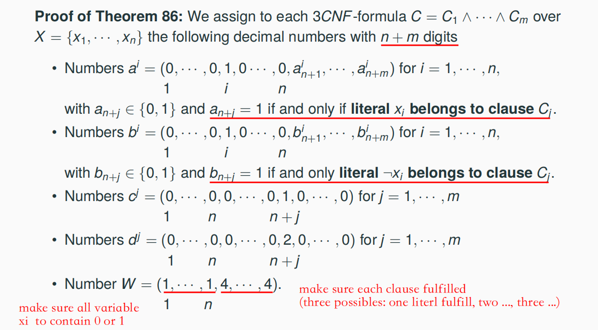
Let L ∈ NP be arbitrarily fixed. We construct for each input x ∈ {0, 1}*a CNF-formula C^x of polynomial size such that x ∈ L ==C^x ∈ SAT
Turing Machines
Extended Hypothesis of Church: each
polynomial time algorithm can be executed on a polynomial time bounded One-tape
Turing machine (for short 1-TM)
- A 1-TM M has one linear tape consisting of a (potentially unbounded) number of register cells, where in each register cell characters from {0, 1, #} can be stored
- At the tape a head is operating which is connected with a CPU
- M is working clockwise on the basis of a TM-program, called state transition
function. In each clock cycle, the machine is in a certain inner state q, and the head is at and reads a character b from a certain register cell. Depending on q and b, the head writes a new letter into this cell, moves to the left or to the right neighbor cell, and changes the inner state
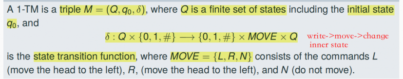
- δ-Instances (q, b; b’, m, q0 ) correspond to TM-commands of type: If M is in state q and reads b then write b’, move the head according to m and change into state q’.
- At the beginning of a computation, M is in initial state q0 and the head is at some
predefined initial position - Instances (q, b; b, N, q) for q ∈ Q and b ∈ {0, 1, #} are called stop instances.
- States q ∈ Q for which (q, b; b, N, q) ∈ δ for all b ∈ {0, 1, #} are called stop states


7.12 The reduction method for showing NP-Completeness
We want to show that a given NP-Problem L is NP-complete.
For that it is sufficient to find an appropriate NP-complete problem L’ (for example, SAT ), and to construct a polynomial reduction g from L’ to L
7.11.1 A Polynomial Reduction from SAT to 3SAT => 3SAT ∈ NPC
3SAT ∈ NPC


7.11.2 A Polynomial Reduction from 3SAT to Clique => Clique ∈ NPC


7.11.3 A Polynomial Reduction from 3SAT to KP* => LP* ∈ NPC

7.11.4 A Polynomial Reduction from KP* to Partition => Partition ∈ NPC


7.11.5 DHC,HC,TSP ∈ NP
3SAT => DHC => HC => TSP
8. Hardnes of General Problems
8.1 NP-Hard
Assume P/=NP: If a decision problem L is NP-complete then L /∈ P
A corresponding concept for general computational problems Π:
Π is called NP-hard if Π ∈ PTIME implies P = NP
8.2 Oracle Algorithms and Turing-Reducibility
We showed NP-completeness by constructing polynomial reductions, a concept applicable only to decision problems. We define Turing-reducibility (Π ≤T Π’), a reducibility concept applicable to general problems Π, Π’
Informally, a Turing reduction from Π to Π’ is a polynomial time algorithm for Π, which has access to a subroutine for Π‘, which on arbitrary inputs x returns immediately a solution y with (x, y) ∈ Π‘
A Π‘-Oracle is a computational device with possibly supernatural computational power. It solves the computational problem Π‘ with maximal efficiency, i.e. for all inputs x the Π’-Oracle returns a solution y with (x, y) ∈ Π‘ in time |x| + |y|
A Π’-Oracle Algorithm for a given computational problem Π‘ is an algorithm which solves Π and has access to an Π’-oracle.
We define Π to be Turing-reducible to Π‘ (Π ≤T Π’), if there is a polynomial time Π‘-oracle algorithm for Π.
The concept of oracle algorithms corresponds to the well-known concept in programming that a given computer program calls a subprogram.
The concept of Turing-Reducibility allows to determine the complexity of a given problem Π relative to another problem Π‘ in the sense of If Π is hard then also Π’ is hard or If Π‘ is easy then also Π is easy.

Polynomial Reductions are special cases of Turing reductions, i.e., from L ≤pol L‘ it
follows that L ≤T L’
For all optimization problems Π, the decisional variant LΠ is Turing reducible to Π
Self Reducibility means that the reverse case is also true, i.e., the optimization variant is Turing-reducible to the (easier looking) decisional variant.
Example: The optimization problem MaxClique (of computing a clique of maximal size in a given input graph G = (V, E)) is Turing-reducible to its decision variant Clique (of deciding if G contains a clique of size at least k).

8.3 An SAT-Oracle Algorithm for SAT.ASSIGNMENT
 SAT.ASSIGNMENT ≤T SAT
8.4 NP-hard, NP-easy, and NP-equivalent Problems
A computational problem Π is called
- NP-hard, if there is an NPC-problem L with L ≤T Π.
- NP-easy, if there is an NP-problem L with Π ≤T L.
- NP-equivalent, if Π is NP-easy and NP-hard.
Let Π NP-hard. Then Π ∈ PTIME -> P = NP.
Let Π NP-easy. Then P = NP -> Π ∈ PTIME.
All NP problems are NP-easy, all NPC-problems are NP-equivalent
Optimization problems, for which the decisional variant is NP-complete, are NP-hard
Optimization problems, which can be Turing-reduced to its decisional variant are NP-easy (MaxClique, MinTSP, MaxKP,… )
8.5 Algorithms for NP-hard Optimization Problems
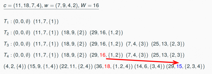
8.5.1 DynamicKP, a Dynamic Algorithm for MaxKP
There is an algorithm for the NP-hard problem MaxKP which needs time O(n·cmax (I)) for each integral input instance I = (n, w1,…, wn, c1, …, cn, W), where cmax (I) = max{ci, i = 1, …, n}


8.4.2 Number Problems and Pseudipolynomial Algorithms
A problem is called number problem if the components of input instances I are natural numbers.
If I is an input instance of a number problem then let Max(I) denote the maximal component of I
Let Π denote a number problem. An algorithm A for Π is called pseudopolynomial if the running time is polynomially bounded in |I| and Max(I).
The NP-hard MaxKP has a pseudopolynomial algorithm
8.5 Strong NP-hard Problems

TSP is strong NP-hard
8.6 Approximation Algorithms for NP-hard Optimization Problems

Many NP-complete optimization problems have polynomial time approximation algorithms which reach a good approximation ratio. In particular,
- Good News: There are NP-hard optimization problems with polynomial time approximation algorithms of constant ratio Ra(n) ∈ O(1) (VertexCover).
- Better News: There are even NP-hard optimization problems with polynomial time approximation algorithms with constant ratio arbitrarily close to one (MaxKP)
- Bad News: There are other NP-hard optimization problems which do not have polynomial time approximation algorithms with constant ratio (MinTSP).
Determining the minimal ratio for which a given NP-hard optimization problem can be approximated in polynomial time is one of the main research topics in modern algorithmics
8.7 Different reductions
- HC ≤pol TSP
- SAT ≤pol 3SAT
- 3SAT ≤pol Clique
- KP* ≤pol KP
- 3SAT ≤pol KP*
- KP* ≤pol Partition
- 3SAP ≤pol DHC ≤pol HC ≤pol TSP
(SAT-ASSIGMENT ≤T SAT)
8.8 NPC problems
The list below contains some well-known problems that are NP-complete when expressed as decision problems.
- Boolean satisfiability problem (SAT)
- the problem of determining if there exists an interpretation that satisfies a given Boolean formula. In other words, it asks whether the variables of a given Boolean formula can be consistently replaced by the values TRUE or FALSE in such a way that the formula evaluates to TRUE
- 3SAT
- Like the satisfiability problem for arbitrary formulas, determining the satisfiability of a formula in conjunctive normal form where each clause is limited to at most three literals.
- Knapsack problem
- The decision problem form of the knapsack problem (Can a value of at least V be achieved without exceeding the weight W?) is NP-complete
- Hamiltonian path problem
- are problems of determining whether a Hamiltonian path (a path in an undirected or directed graph that visits each vertex exactly once). The Hamiltonian cycle problem is a special case of the traveling salesman problem, obtained by setting the distance between two cities to one if they are adjacent and two otherwise, and verifying that the total distance traveled is equal to n (if so, the route is a Hamiltonian circuit; if there is no Hamiltonian circuit then the shortest route will be longer).
- Travelling salesman problem (decision version)
- where given a length L, the task is to decide whether the graph has a tour of at most L
- Subgraph isomorphism problem
- a computational task in which two graphs G and H are given as input, and one must determine whether G contains a subgraph that is isomorphic to H. Subgraph isomorphism is a generalization of both the maximum clique problem and the problem of testing whether a graph contains a Hamiltonian cycle, and is therefore NP-complete
- Subset sum problem SSP
- there is a multiset S of integers and a target-sum T, and the question is to decide whether any subset of the integers sum to precisely T.
- The variant in which all inputs are positive, and the target sum is exactly half the sum of all inputs. This special case of SSP is known as the partition problem.
- SSP is a special case of the knapsack problem and of the multiple subset sum problem.
- Clique problem
- testing whether a graph contains a clique larger than a given size
- Vertex cover problem
- a vertex cover (sometimes node cover) of a graph is a set of vertices that includes at least one endpoint of every edge of the graph
- INSTANCE: Graph G and positive integer k
QUESTION: Does G have a vertex cover of size at most k?
- Independent set problem
- an independent set, stable set, coclique or anticlique is a set of vertices in a graph, no two of which are adjacent. Equivalently, each edge in the graph has at most one endpoint in S
- Dominating set problem
- Graph coloring problem
8.9 NP-hard Problems
- Travelling salesman problem TSP (combinatorial optimization version)
- Given a list of cities and the distances between each pair of cities, what is the shortest possible route that visits each city exactly once and returns to the origin city?
- Minimum vertex cover (optimization problem)
- The minimum vertex cover problem is the optimization problem of finding a smallest vertex cover in a given graph.
INSTANCE: Graph G
OUTPUT: Smallest number k such that G has a vertex cover of size k
- The minimum vertex cover problem is the optimization problem of finding a smallest vertex cover in a given graph.
- subset sum problem
- SAT optimization version
8.10 Strongly NP-hard Problems
- Maximum independent set problem
- Bin packing
- a list of objects of specific sizes and a size for the bins that must contain the objects—these object sizes and bin size are numerical parameters.
- TSP Optimization problem


 770
770


 被折叠的 条评论
为什么被折叠?
被折叠的 条评论
为什么被折叠?
 到【灌水乐园】发言


