Data Mining2复习笔记1 Data Preprocessing

1. Data Preprocessing

1.1 Errors in Data

Source

• malfunctioning sensors
• errors in manual data processing (e.g., twisted digits)
• storage/transmission errors
• encoding problems, misinterpreted file formats
• bugs in processing code
• …

Simple remedy
remove data points outside a given interval (requires some domain knowledge)

Typical Examples
remove temperature values outside -30 and +50 °C
remove negative durations
remove purchases above 1M Euro

Advanced remedies
automatically find suspicious data points (Anomaly Detection)

1.2 Missing Values

Possible reasons

• Failure of a sensor
• Data loss
• Information was not collected
• Customers did not provide their age, sex, marital status, …
• …

Treatments

• Ignore records with missing values in training data
• Replace missing value with…
  • default or special value (e.g., 0, “missing”)
  • average/median value for numerics
  • most frequent value for nominals
• Try to predict missing values:
  • handle missing values as learning problem
  • target: attribute which has missing values
  • training data: instances where the attribute is present
  • test data: instances where the attribute is missing

Note: values may be missing for various reasons, and more importantly: at random vs. not at random

Examples for not random

• Non-mandatory questions in questionnaires
• Values that are only collected under certain conditions
• Values only valid for certain data sub-populations
• Sensors failing under certain conditions

In those cases, averaging and imputation causes information loss -> “missing” can be information!

Missing Values vs. Missing Observations
Missing values: Typically single fields in a record + Can be handled with imputation etc.

Missing observations: Entire records missing + Various forms (Selection bias, Missing values in time series)

1.3 Unbalanced Distribution

Example: learn a model that recognizes HIV, given a set of symptoms.
Data set: records of patients who were tested for HIV
Class distribution: 99.9% negative, 0.01% positive

Learn a decision tree
Purity measure: Gini index

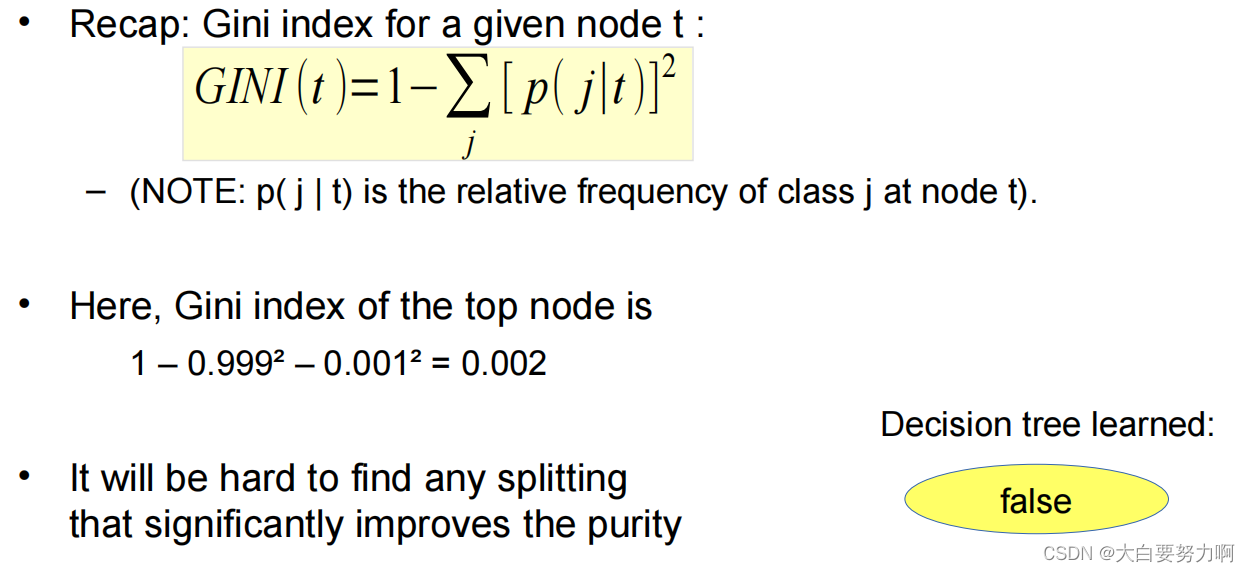
Model has very high accuracy, but 0 recall/precision on positive class, which is what we were interested in.

Remedy
re-balance dataset for training but evaluate on unbalanced dataset!

Resampling Unbalanced Data
Two conflicting goals
(1) use as much training data as possible
(2) use as diverse training data as possible

Strategies
(1) Downsampling larger class - conflicts with goal 1
(2) Upsampling smaller class - conflicts with goal 2

Consider an extreme example: 1,000 examples of class A, 10 examples of class B

Downsampling: does not use 990 examples
Upsampling: creates 100 copies of each example of B, likely for the classifier to simply memorize the 10 B cases

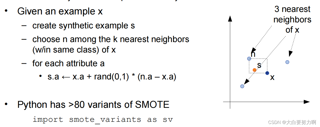
(3) Resampling with SMOTE (Synthetic Minority Over Sampling Technique) - creates synthetic examples of minority class

Stratification vs. changing the distribution

• Stratified sampling: keep class distribution
• Upsampling and downsampling: balance class distribution
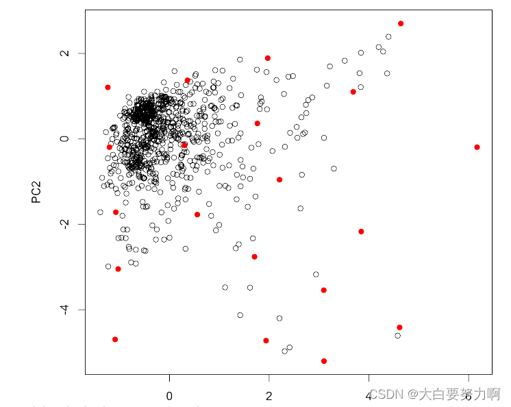
• Kennard-Stone sampling tries to select heterogenous points

Kennard-Stone Sampling

1. Compute pairwise distances of points
2. Add points with largest distance from one another
3. While target sample size not reached
   1. For each candidate, find smallest distance to any point in the sample
   2. Add candidate with largest smallest distance

This guarantees that heterogeneous data points are added, i.e., sample gets more diverse. It includes more corner cases but potentially also more outliers. Distribution may be altered

Pro: a lot of rare cases covered
Con: original distribution gets lost

Sampling Strategies and Learning Algorithms
There are interaction effects. Some learning algorithms rely on distributions, e.g., Naive Bayes –> usually, stratified sampling works better. Some rely less on distributions, e.g., Decision Trees -> may work better if they see more corner cases

Often, the training data in a real-world project is already a sample, e.g., sales figures of last month -> to predict the sales figures for the rest of the year
How representative is that sample? What if last month was December? Or February?

Effect known as selection bias
Example: phone survey with 3,000 participants, carried out Monday, 9-17
Thought experiment: effect of selection bias for prediction,
e.g., with a Naive Bayes classifier

1.4 False Predictors

~100% accuracy are a great result and a result that should make you suspicious!
False predictor: target variable was included in attributes

Example: mark<5 → passed=true; sales>1000000 → bestseller=true

Recognizing False Predictors
(1) By analyzing models - rule sets consisting of only one rule; decision trees with only one node
Process: learn model, inspect model, remove suspect, repeat until the accuracy drops

(2) By analyzing attributes - compute correlation of each attribute with label; correlation near 1 (or -1) marks a suspect

Caution: there are also strong (but not false) predictors – it’s not always possible to decide automatically

1.5 Unsupported Data Types

Not every learning operator supports all data types
– some (e.g., ID3) cannot handle numeric data
– others (e.g., SVM) cannot nominal data
– dates are difficult for most learners

solutions
– convert nominal to numeric data
– convert numeric to nominal data (discretization, binning)
– extract valuable information from dates

1.5.1 Conversion

1.5.1.1 Binary to Numeric

Binary fields -> 0 & 1

1.5.1.2 Conversion: Nominal to Numeric

Multi-valued, unordered attributes with small no. of values -> one hot encoding: N binary or 0/1 variables, only one is “hot” (true or 1)

1.5.1.3 Conversion: Ordinal to Numeric

Some nominal attributes incorporated an order -> Ordered attributes (e.g. grade) can be converted to numbers preserving natural order.
Using such a coding schema allows learners to learn valuable rules

1.5.1.4 Conversion: Nominal to Numeric

manual, with background knowledge (e.g. group US states into west, mideast, northeast, south)
use binary attributes, then apply dimensionality reduction

1.5.2 Discretization

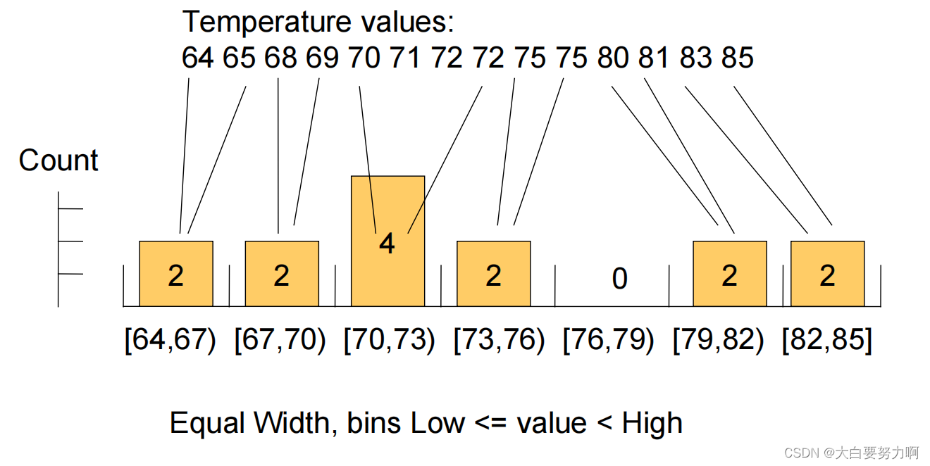
1.5.2.1 Discretization: Equal-width

1.5.2.2 Discretization: Equal-height

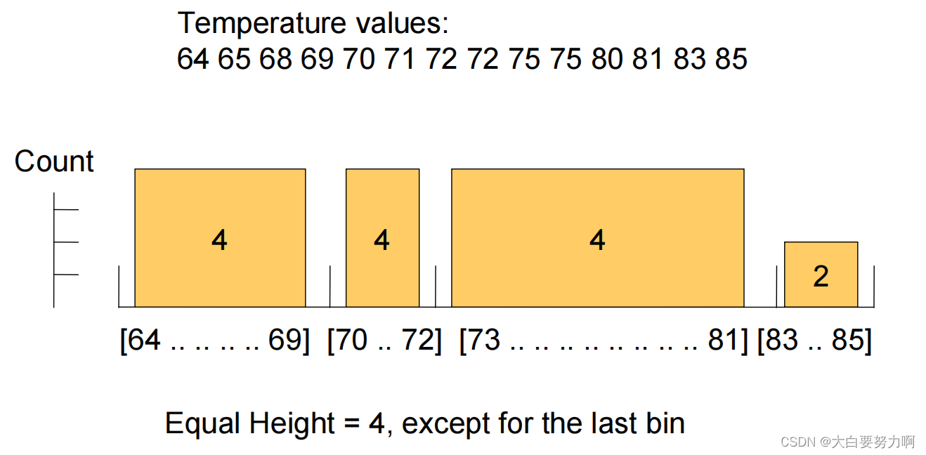
1.5.2.3 Discretization: Entropy

Top-down approach
Tries to minimize the entropy in each bin
Entropy (x are all the attribute values):

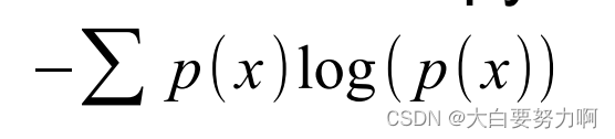
Goal: make intra-bin similarity as high as possible
a bin with only equal values has entropy=0

Algorithm

1. Split into two bins so that overall entropy is minimized
2. Split each bin recursively as long as entropy decreases significantly

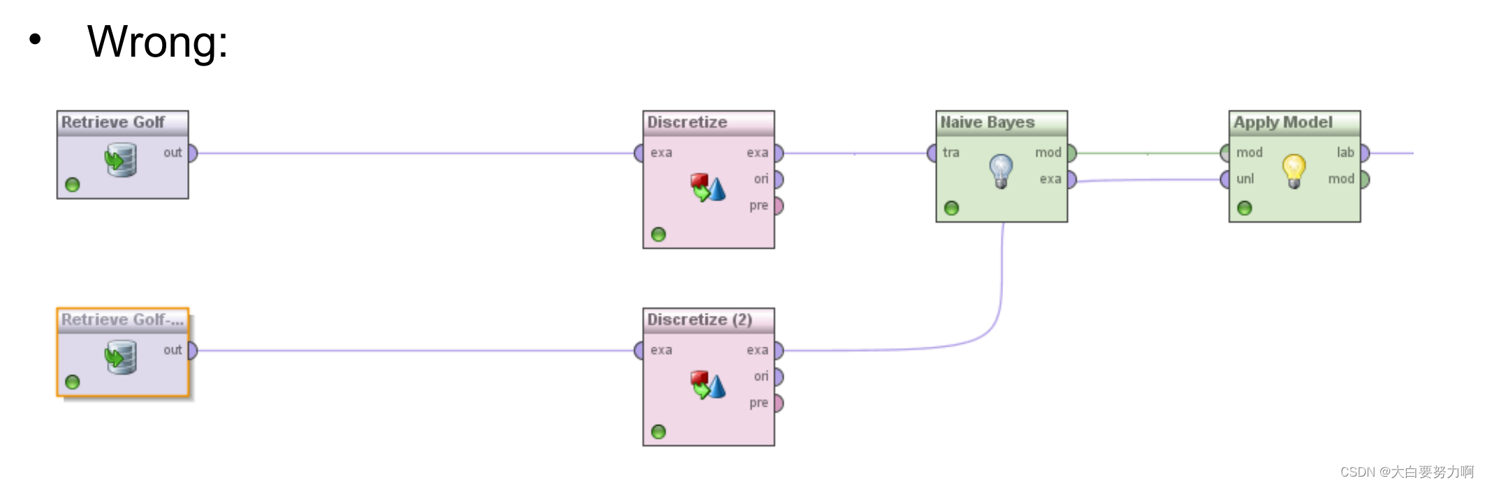
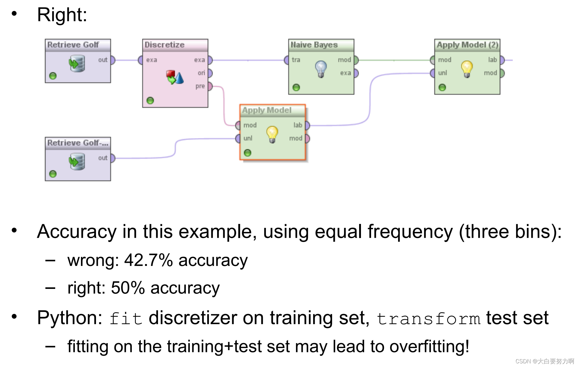
1.5.2.4 Trading and Test Data

Training and test data have to be equally discretized!

Learned model:
– income=high → give_credit=true
– income=low → give_credit=false

Applying model:
income=low has to have the same semantics on training and test data!
Naively applying discretization will lead to different ranges!

1.5.2.5 Semi-supervised Learning

Labeling data with ground truth can be expensive
Example: Medical images annotated with diagnoses by medical experts

Typical case:
Smaller subset of labeled data (gold standard). Larger subset of unlabeled data

Semi-supervised learning: Tries to combine both types of data

Semi-supervised learning can be applied to discretization
Learn distribution of an attribute on larger dataset → find better bins

1.5.3 Dealing with Data Attributes

Dates (and times) can be formatted in various ways
first step: normalize and parse

Further Datatypes: Text & Multi-modal data: Images, Videos, Audio
Typically, encoders are used to create (numeric) representations
from such data

High Dimensionality
Datasets with large number of attributes
Examples: text classification, image classification, genome classification, …
(not only a) scalability problem, e.g., decision tree: search all attributes for determining one single split

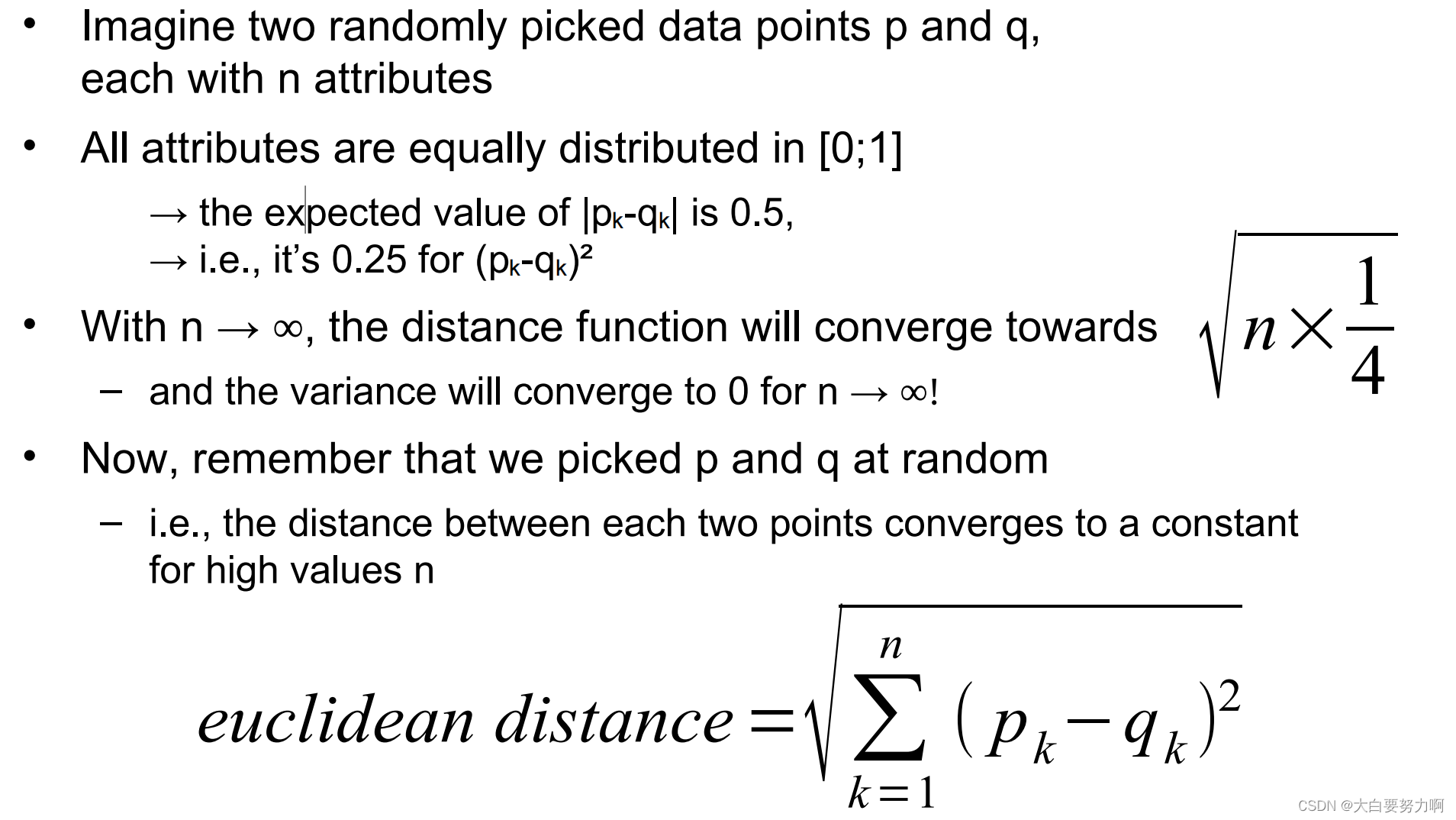
1.5.4 Curse of Dimensionality

Learning models gets more complicated in high-dimensional spaces
Higher number of observations are needed -> For covering a meaningful number of combinations (“Combinatorial Explosion”))

Distance functions collapse
i.e., all distances converge in high dimensions
Nearest neighbor classifiers are no longer meaningful

Why does Euclidean Distance Collapse维度灾难?
高维数据的距离都会变得无意义，因为彼此之间都非常远并收敛于一个值，变化趋于0，此时基于距离的算法像KNN这种会失效。

1.6 Feature Subset Selection

Preprocessing step
Idea: only use valuable features

Basic heuristics: remove nominal attributes…
– which have more than p% identical values
example: millionaire=false
– which have more than p% different values
• example: names, IDs

Basic heuristics: remove numerical attributes
– which have little variation, i.e., standard deviation <s

Basic Distinction: Filter vs. Wrapper Methods
Filter methods
Use attribute weighting criterion, e.g., Chi², Information Gain, … -> Select attributes with highest weights
Fast (linear in no. of attributes), but not always optimal

Remove redundant attributes (e.g., temperature in °C and °F, textual features “Barack” and “Obama”)
compute pairwise correlations between attributes -> remove highly correlated attributes

Recap:
Naive Bayes requires independent attributes
Will benefit from removing correlated attributes

Wrapper methods
Use classifier internally -> Run with different feature sets -> Select best feature set

Advantages: Good feature set for given classifier

Disadvantages: Expensive (naively: at least quadratic in number of attributes) & Heuristics can reduce number of classifier runs

Further approaches

• Brute Force search
• Evolutionary algorithms

Trade-off

• simple heuristics are fast but may not be the most effective
• brute-force is most effective but the slowest
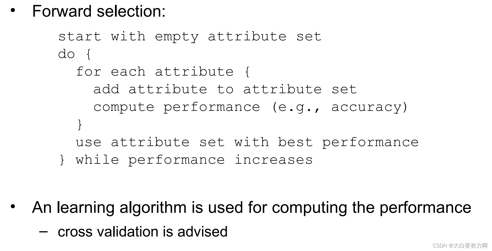
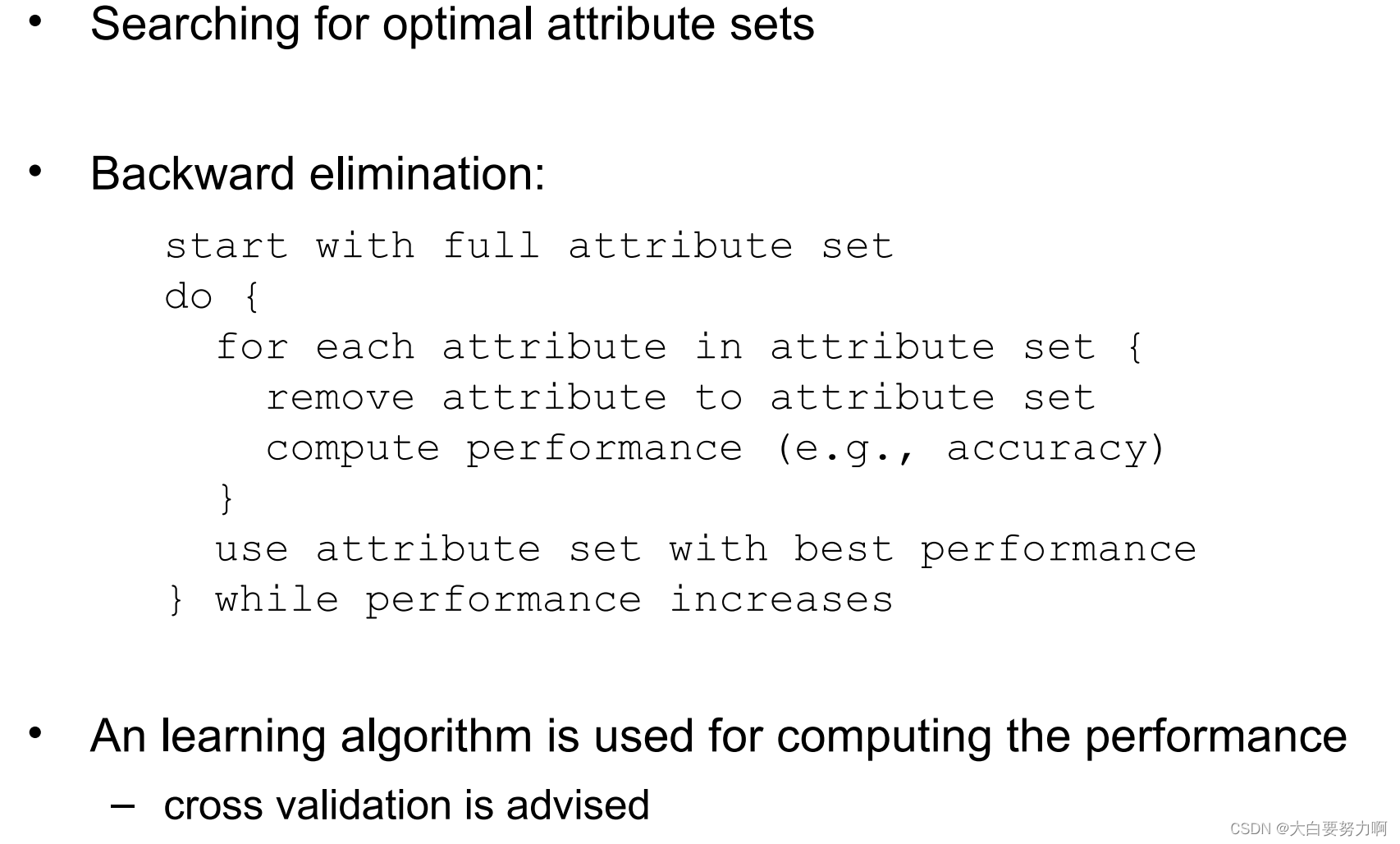
• forward selection, backward elimination, and evolutionary algorithms are often a good compromise

Overfitting can happen with feature subsect selection, too
Here, name seems to be a useful feature, …but is it?

Remedies: Hard for filtering methods
• e.g., name has highest information gain!

Wrapper methods: use cross validation inside!

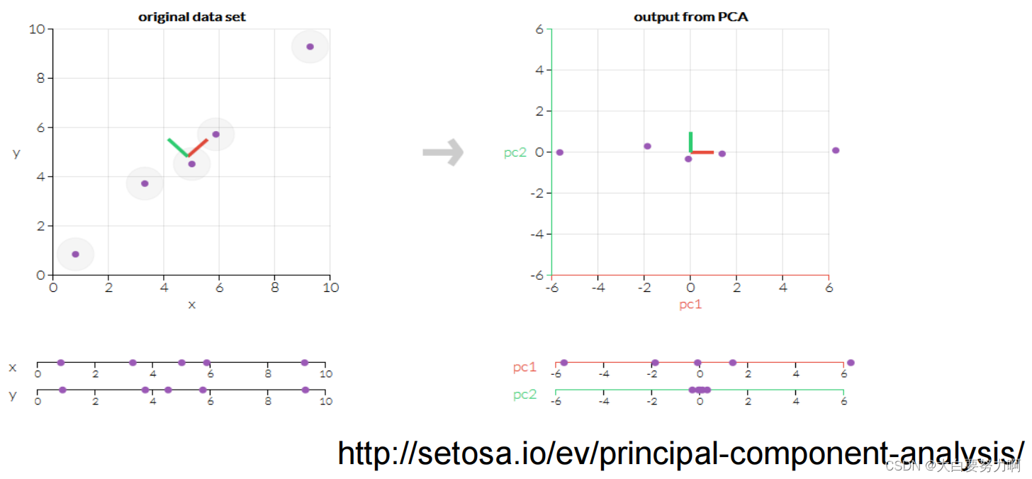
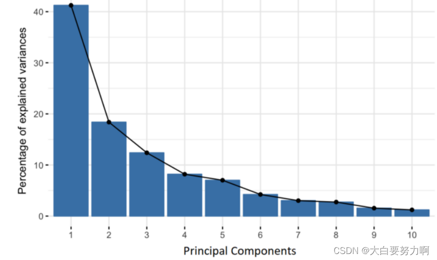
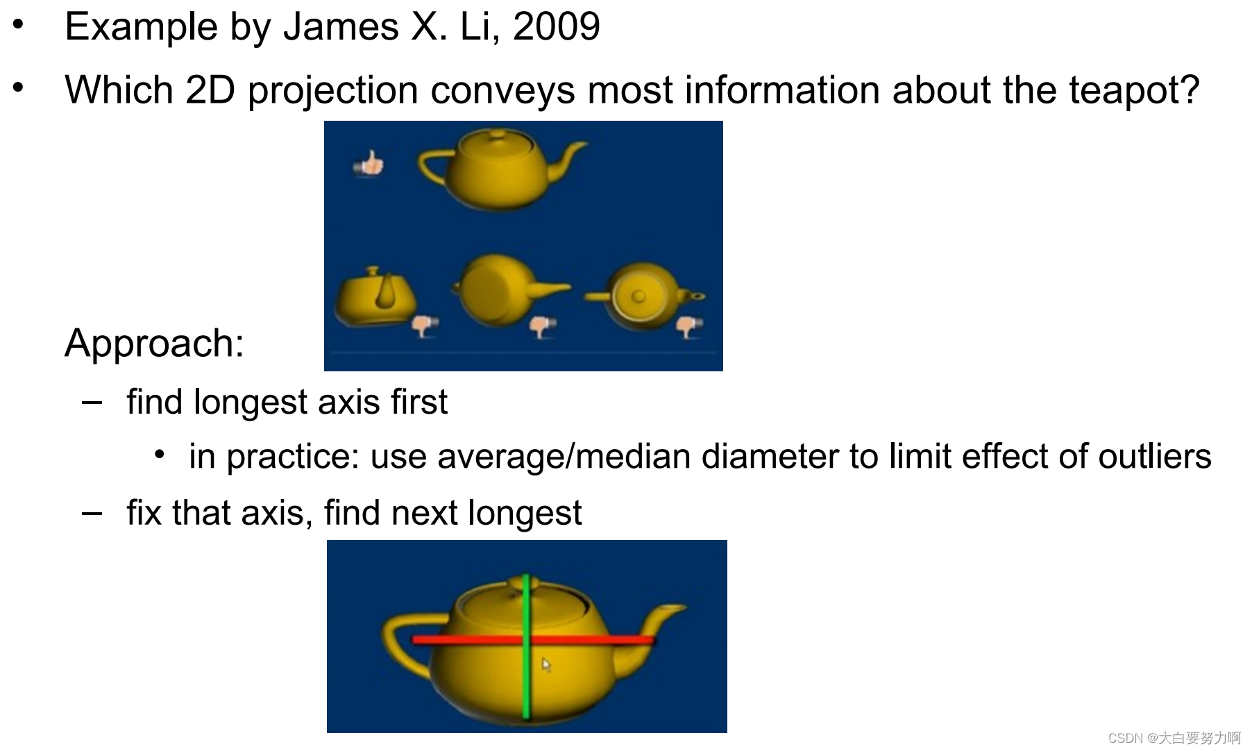
Principal Component Analysis (PCA)
PCA creates a (smaller set of) new attributes

• artificial linear combinations of existing attributes
• as expressive as possible

Idea: transform coordinate system so that each new coordinate (principal component) is as expressive as possible
expressivity: variance of the variable
the 1st, 2nd, 3rd… PC should account for as much variance as possible, further PCs can be neglected

Principal components are linear combinations of the existing features

General approach
(1) The first component should have as much variance as possible
(2)The subsequent ones should also have as much variance as possible and be perpendicular to the first one

PCA can be seen as an encoder
It computes a new representation (encoding) from an existing one

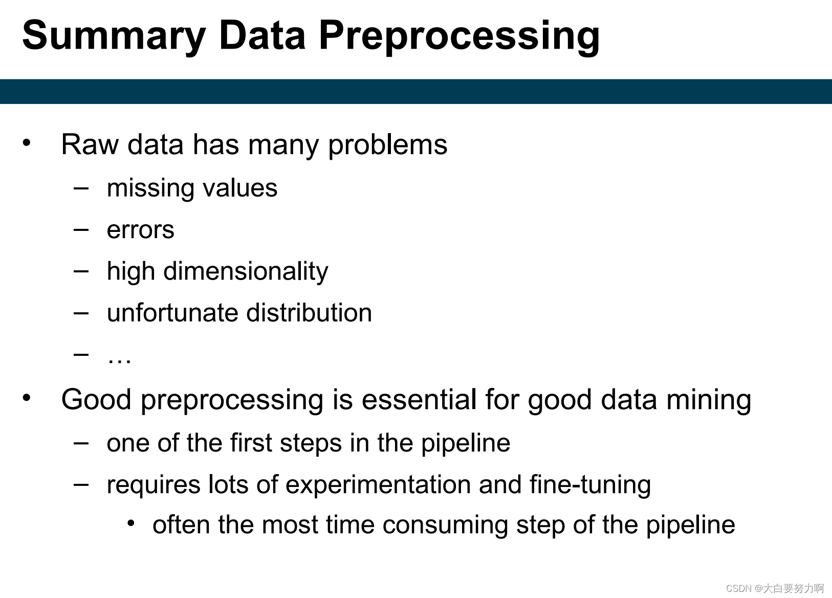
1.7 Summary