Data Mining2复习笔记5 - Anomaly Detection

5. Anomaly Detection

Also known as “Outlier Detection”. Automatically identify data points that are somehow different from the rest

Working assumption: There are considerably more “normal” observations than “abnormal” observations (outliers/anomalies) in the data

Challenges
How many outliers are there in the data?
What do they look like?
Method is unsupervised: Validation can be quite challenging (just like for clustering)

Recap: Errors in Data
Sources: malfunctioning sensors | errors in manual data processing (e.g., twisted digits) | storage/transmission errors | encoding problems, misinterpreted file formats | bugs in processing code | …

Simple remedy: remove data points outside a given interval (this requires some domain knowledge)

Advanced remedies: automatically find suspicious data points

Applications: Data Preprocessing
Data preprocessing: removing erroneous data & removing true, but useless deviations

Example: tracking people down using their GPS data
GPS values might be wrong
person may be on holidays in Hawaii

Applications: Credit Card Fraud Detection
Goal: identify unusual transactions -> possible attributes: location, amount, currency, …

Applications: Hardware Failure Detection
Applications: Stock Monitoring

Cautions: Errors vs. Natural Outliers

Errors, Outliers, Anomalies, Novelties…
What are we looking for?
Wrong data values (errors)
Unusual observations (outliers or anomalies)
Observations not in line with previous observations (novelties)

Unsupervised Setting:
Data contains both normal and outlier points
Task: compute outlier score for each data point

Supervised setting:
Training data is considered normal
Train a model to identify outliers in test dataset

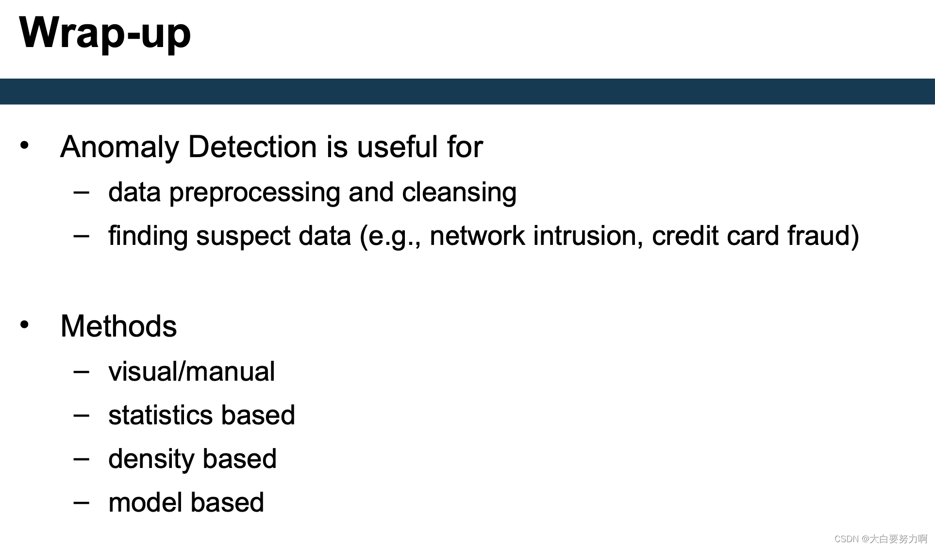
Methods for Anomaly Detection
Graphical: Look at data, identify suspicious observations
Statistic: Identify statistical characteristics of the data, e.g., mean, standard deviation. Find data points which do not follow those characteristics
Density-based: Consider distributions of data & Dense regions are considered the “normal” behavior
Model-based: Fit an explicit model to the data & Identify points which do not behave according to that model

Anomaly Detection Schemes
General Steps

1. Build a profile of the “normal” behavior
   Profile can be patterns or summary statistics for the overall population
2. Use the “normal” profile to detect anomalies
   Anomalies are observations whose characteristics differ significantly from the normal profile

Types of anomaly detection schemes
(1) Graphical & Statistical-based
(2) Distance-based
(3) Model-based

5.1 Graphical Approaches

Boxplot (1-D), Scatter plot (2-D), Spin plot (3-D)
Limitations: Time consuming & Subjective

Convex Hull Method
Extreme points are assumed to be outliers
Use convex hull method to detect extreme values

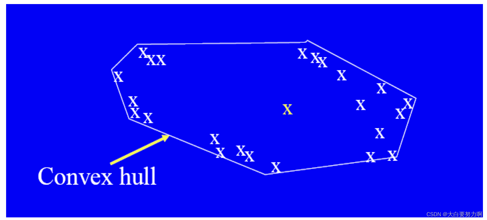
What if the outlier occurs in the middle of the data?

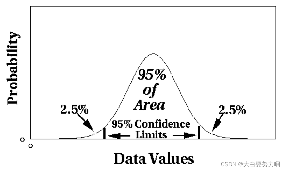
5.2 Statistical Approaches

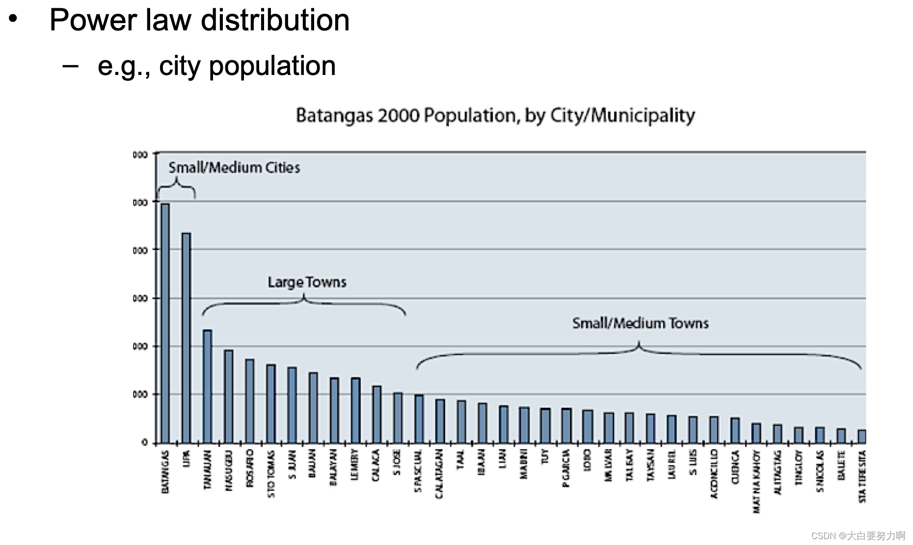
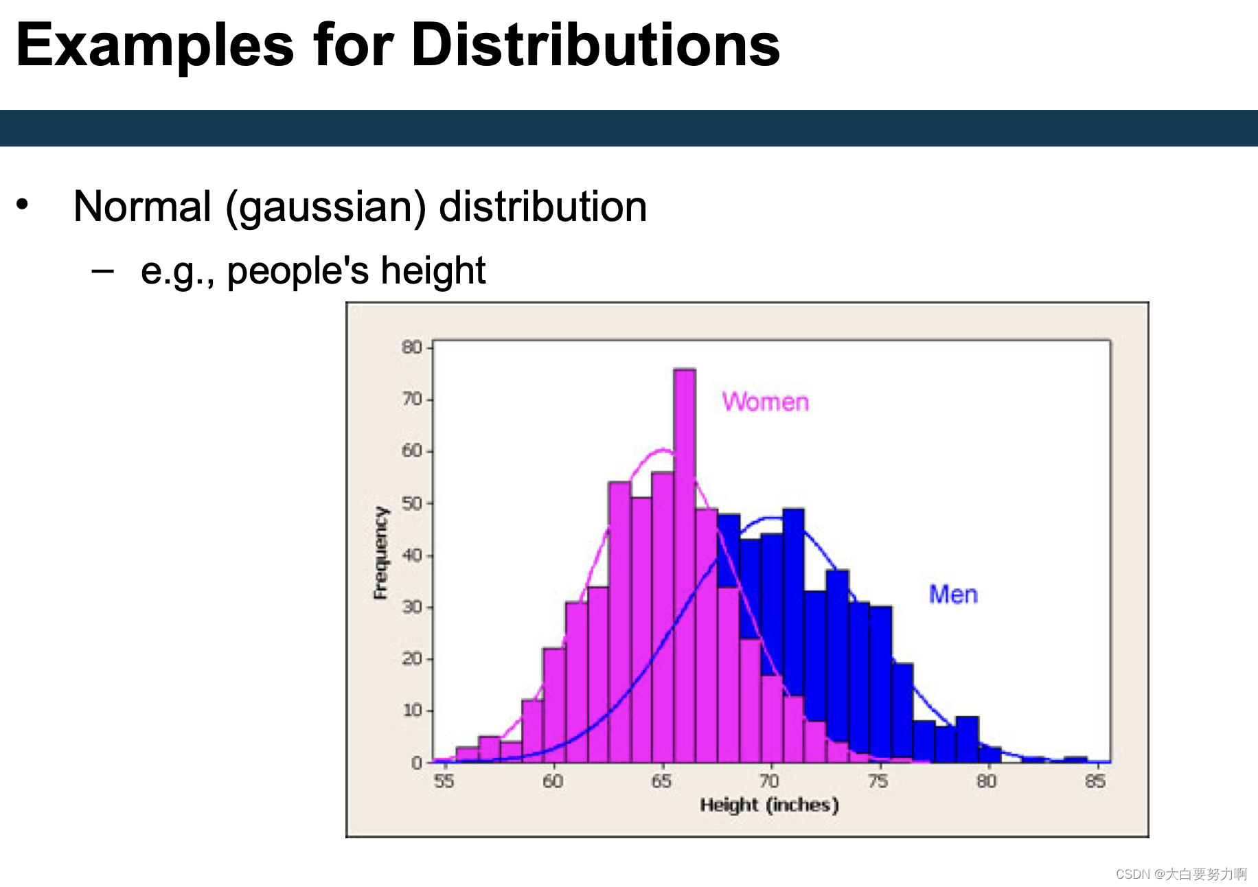
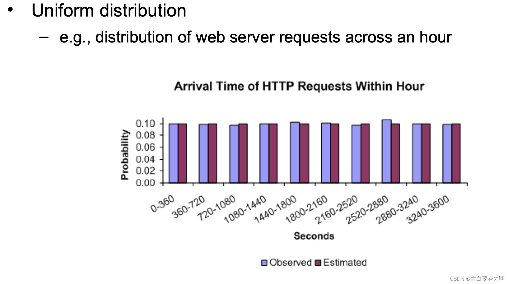
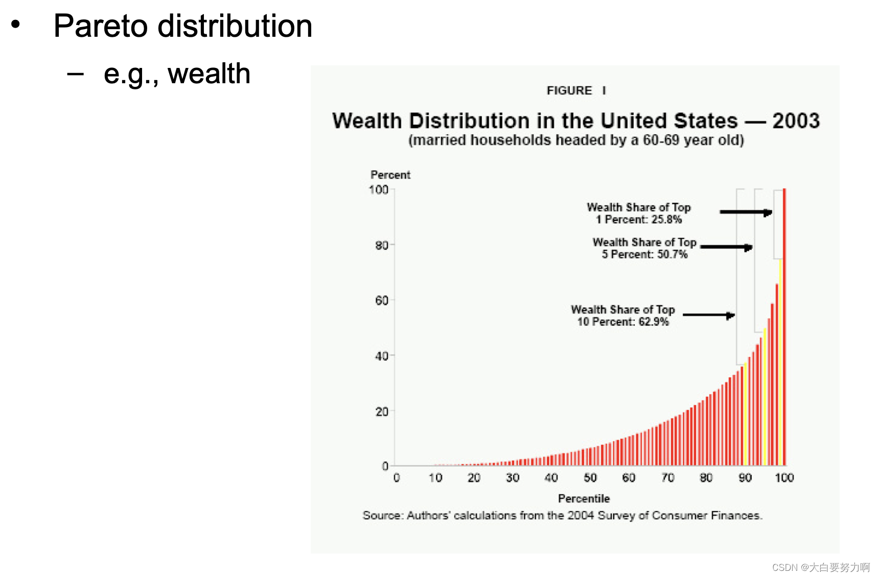
Assume a parametric model describing the distribution of the data (e.g., normal distribution)

Apply a statistical test that depends on

• Data distribution
• Parameter of distribution (e.g., mean, variance)
• Number of expected outliers (confidence limit)

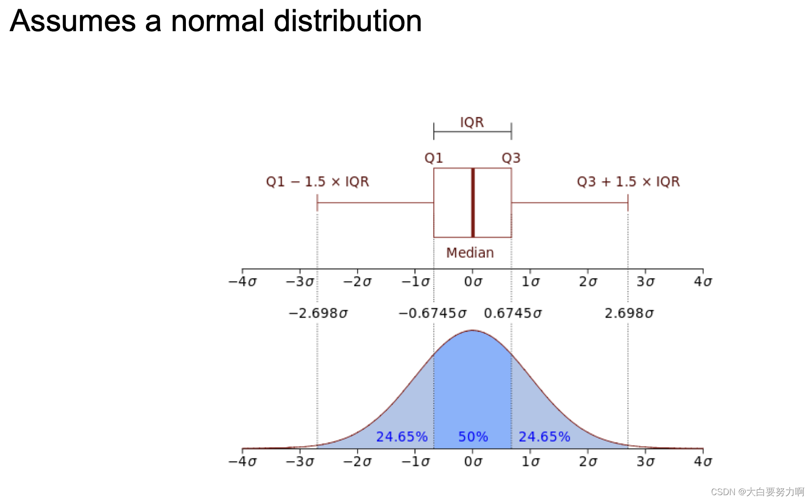
5.2.1 Interquartile Range

Divides data in quartiles
Definitions:
Q1: x≥Q1 holds for 75% of all x
Q3: x≥Q3 holds for 25% of all x
IQR = Q3-Q1

Outlier detection: All values outside [median-1.5IQR ; median+1.5IQR]

Example:
0,1,1,3,3,5,7,42 → median=3, Q1=1, Q3=7 → IQR = 6
Allowed interval: [3-1.56 ; 3+1.56] = [-6 ; 12]
Thus, 42 is an outlier

5.2.2 Median Absolute Deviation (MAD)

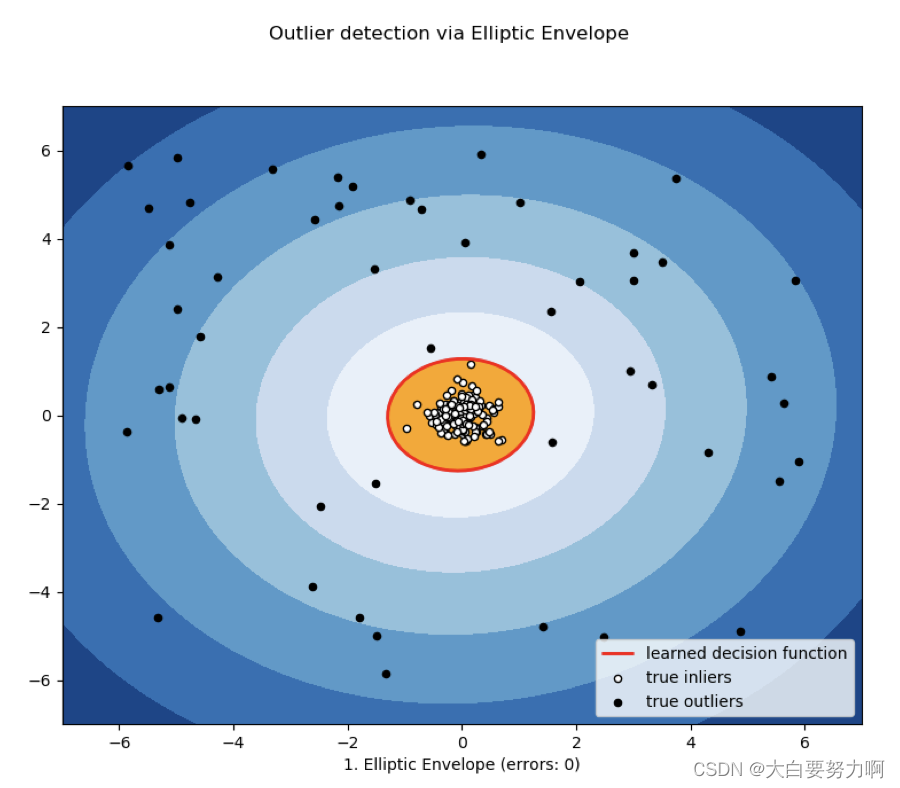
5.2.3 Fitting Elliptic Curves

Multi-dimensional datasets can be seen as following a normal distribution on each dimension. The intervals in one-dimensional cases become elliptic curves.

Limitations
Most of the tests are for a single attribute (called: univariate)
For high dimensional data, it may be difficult to estimate the true distribution
In many cases, the data distribution may not be known – e.g., IQR Test: assumes Gaussian distribution

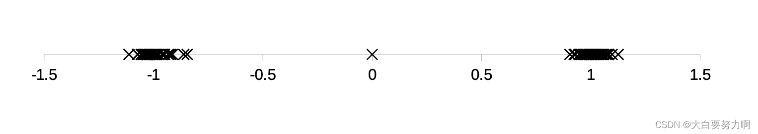
Outliers vs. Extreme Values
So far, we have looked at extreme values only. But outliers can occur as non-extremes. In that case, methods like IQR fail.

5.3 Distance-based Approaches

Data is represented as a vector of features
Various approaches: Nearest-neighbor based, Density based, Clustering based, and Model based

5.3.1 Nearest-Neighbor Based Approach

Compute the distance between every pair of data points
There are various ways to define outliers:

1. Data points for which there are fewer than p neighboring points within a distance D
2. The top n data points whose distance to the kth nearest neighbor is greatest
3. The top n data points whose average distance to the k nearest neighbors is greatest

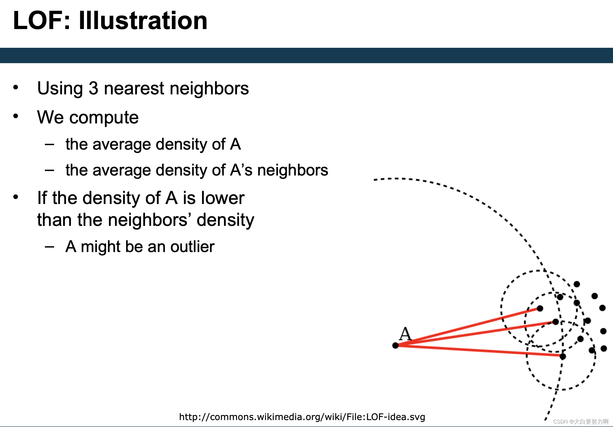
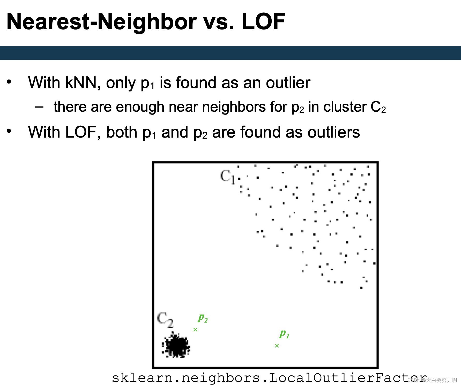
5.3.2 Density based Approach

For each point, compute the density of its local neighborhood
if that density is higher than the average density, the point is in a cluster
if that density is lower than the average density, the point is an outlier

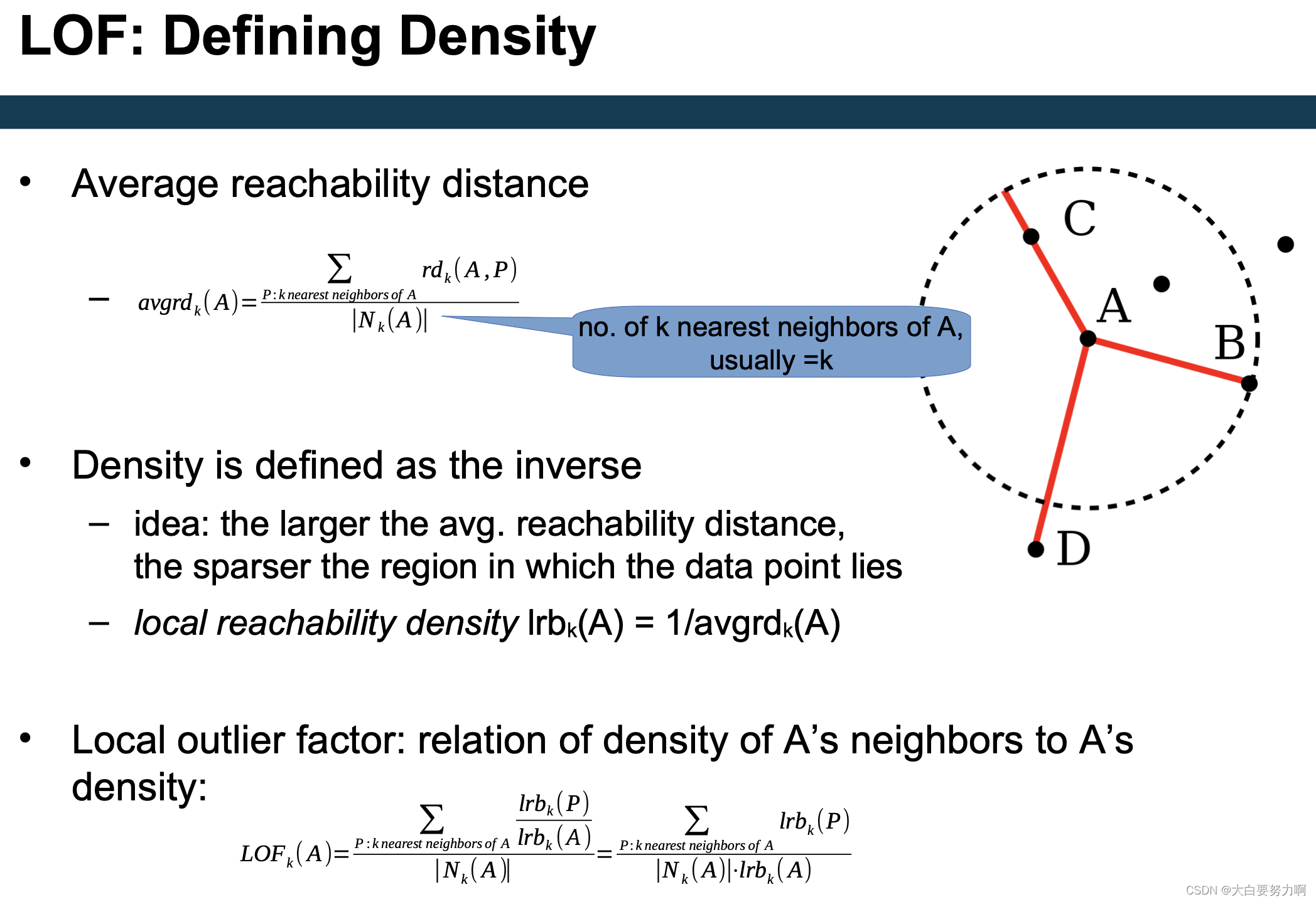
5.3.2.1 LOF

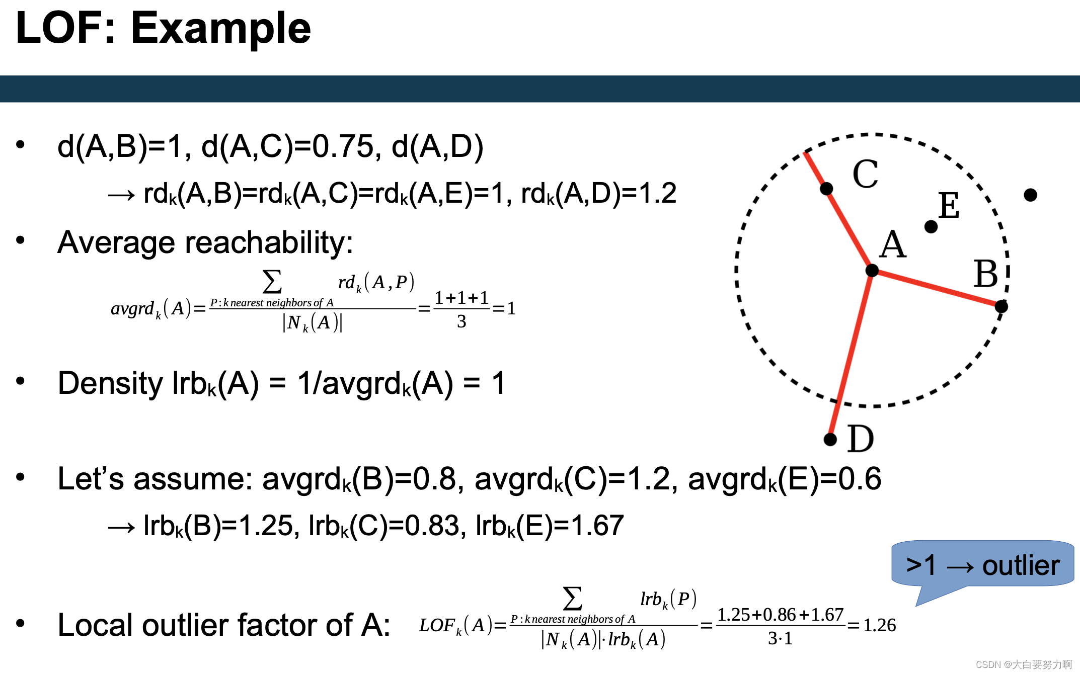
Compute local outlier factor (LOF) of a point A: ratio of average density of A’s neighbors to density of point A
Outliers are points with large LOF value (typical: larger than 1)

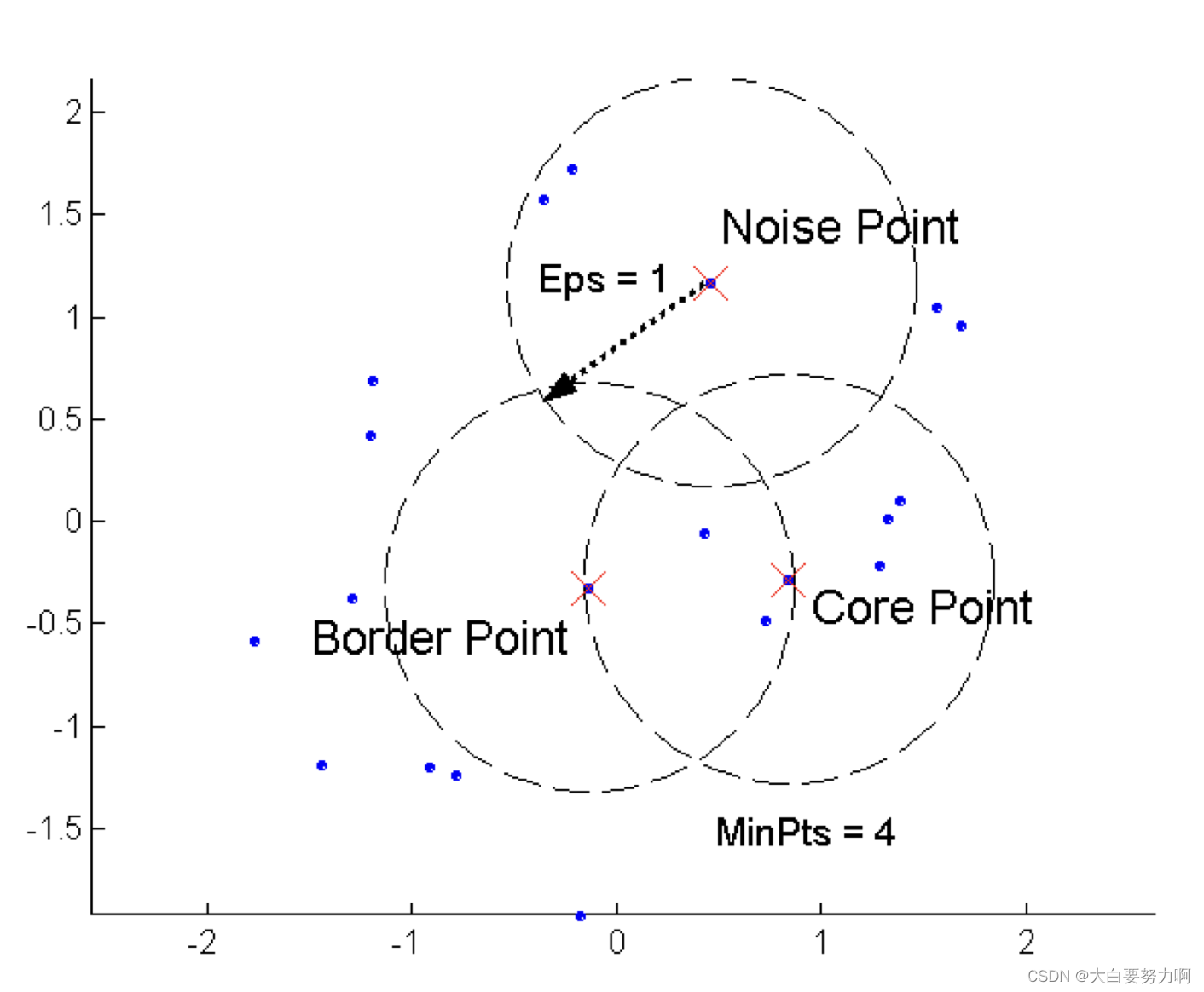
5.3.2.2 DBSCAN

DBSCAN is a density-based algorithm
Density = number of points within a specified radius (Eps)
Divides data points in three classes:
(1) A point is a core point if it has more than a specified number of points (MinPts) within Eps. These are points that are at the interior of a cluster
(2) A border point has fewer than MinPts within Eps, but is in the neighborhood of a core point
(3) A noise point is any point that is not a core point or a border point

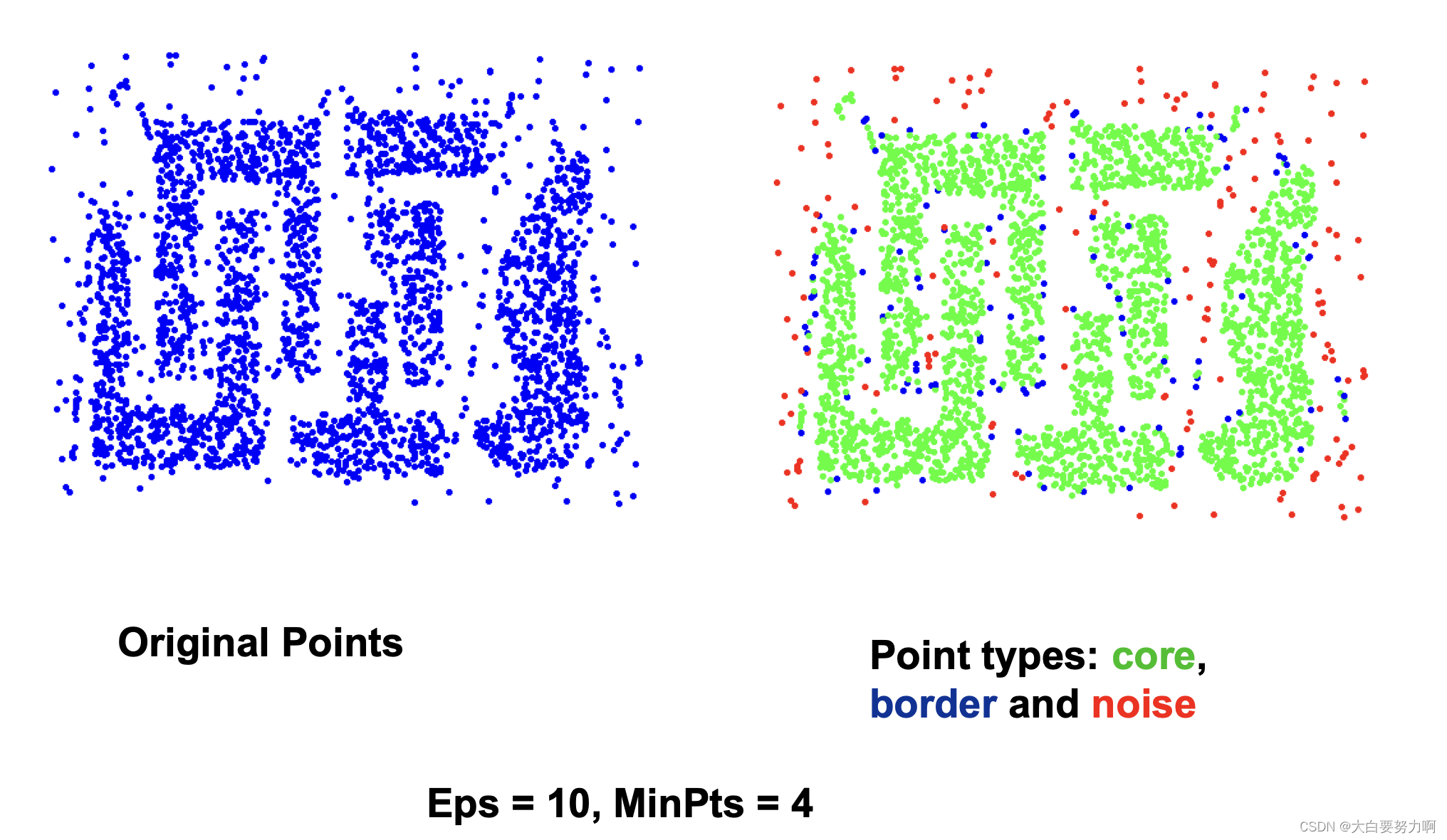
DBSCAN for Outlier Detection
DBSCAN directly identifies noise points. These are outliers not belonging to any cluster.

5.4 Clustering based Approach

Basic idea:
Cluster the data into groups of different density -> Choose points in small cluster as candidate outliers -> Compute the distance between candidate points and non-candidate clusters -> If candidate points are far from all other non-candidate points, they are outliers

5.4.1 Clustering-based Local Outlier Factor

Idea: anomalies are data points that are in a very small cluster or far away from other clusters
CBLOF is run on clustered data: assigns a score based on the size of the cluster a data point is in the distance of the data point to the next large cluster

General process: run a clustering algorithm (of your choice) -> apply CBLOF

5.4.2 PCA and Reconstruction Error

Recap: PCA tries to capture most dominant variations in the data – those can be seen as the “normal” behavior

Reconstruct original data point by inversing PCA
close to original: normally behaving data point
far from original: unnormally behaving data point

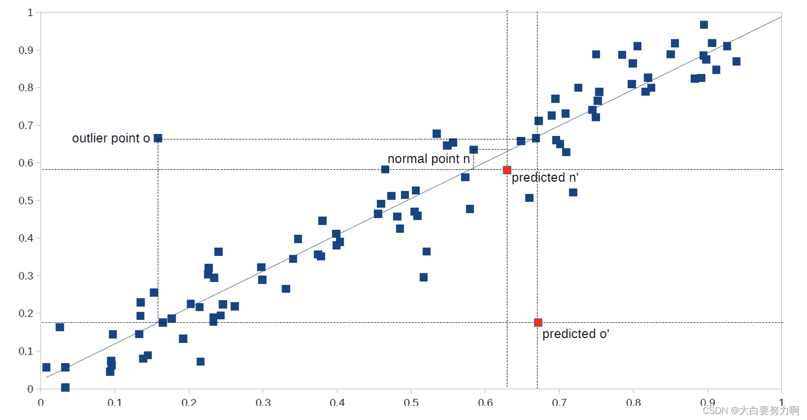
5.5 Model based Approach

Idea: there is a model underlying the data – Data points deviating from the model are outliers.

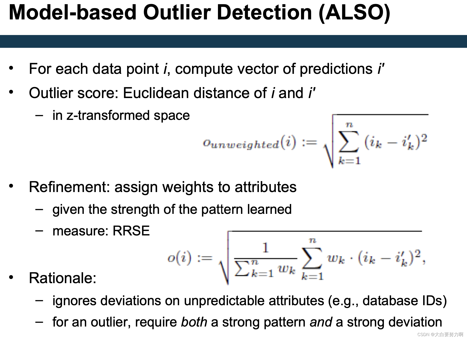
5.5.1 ALSO (Attribute-wise Learning for Scoring Outliers)

Learn a model for each attribute given all other attributes
Use model to predict expected value
Deviation between actual and predicted value → outlier

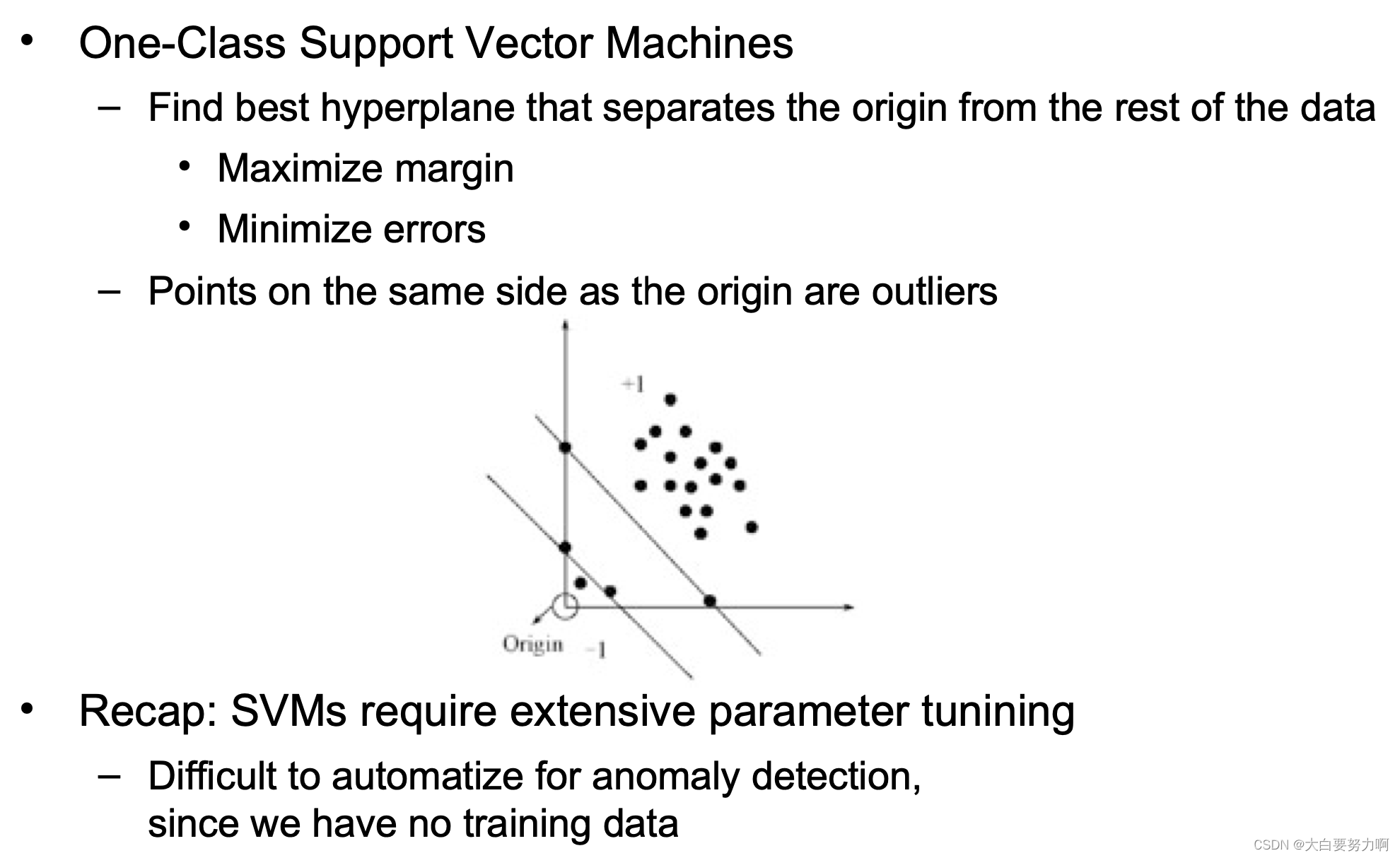
5.5.2 One-Class Support Vector Machines

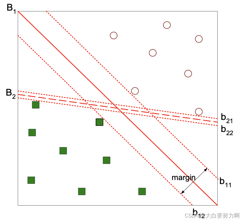
Recap: Support Vector Machines
Find a maximum margin hyperplane to separate two classes
Use a transformation of the vector space
Thus, non-linear boundaries can be found

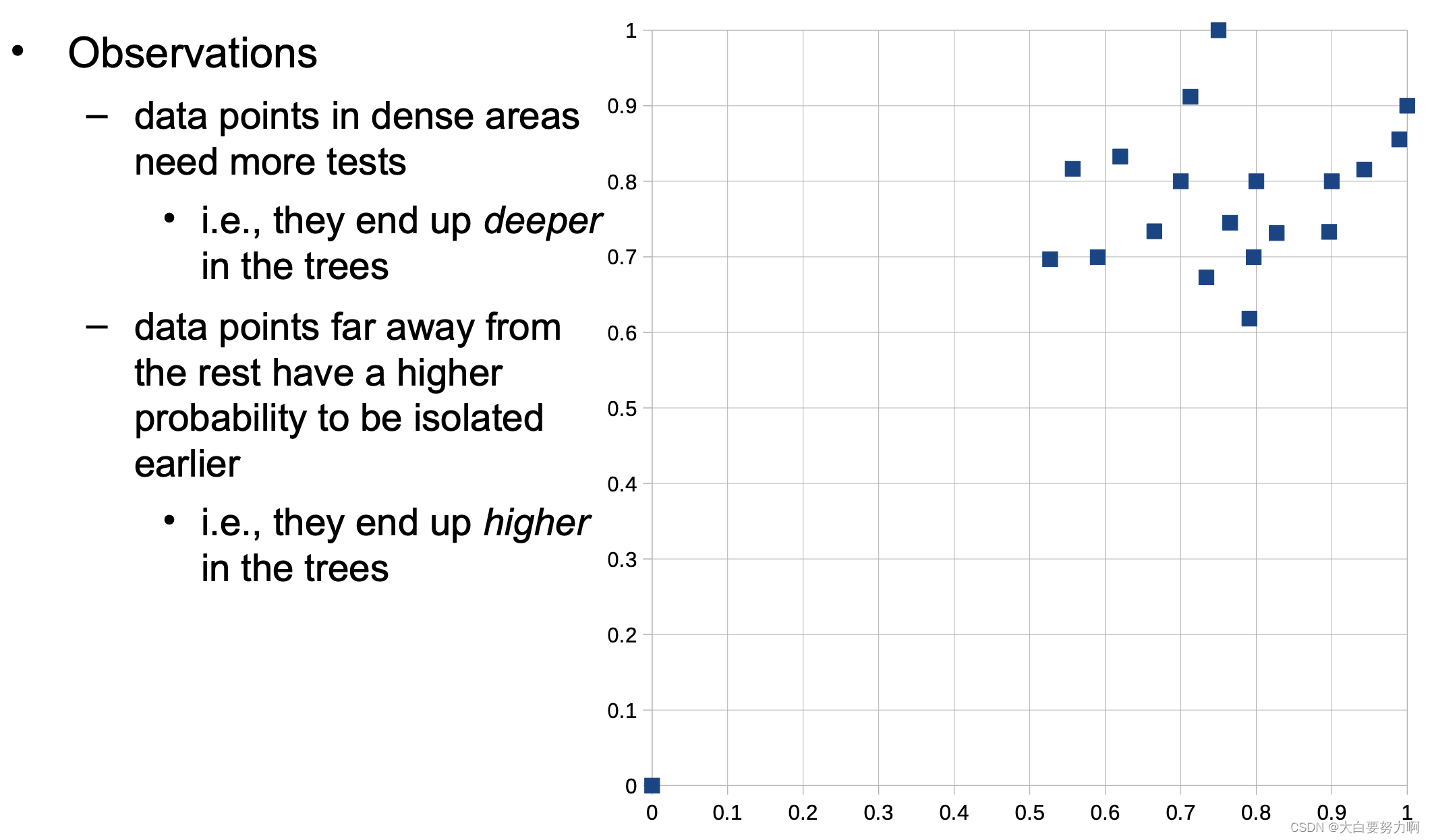
5.5.3 Isolation Forests

Isolation tree: a decision tree that has only leaves with one example each
Isolation forests: train a set of random isolation trees
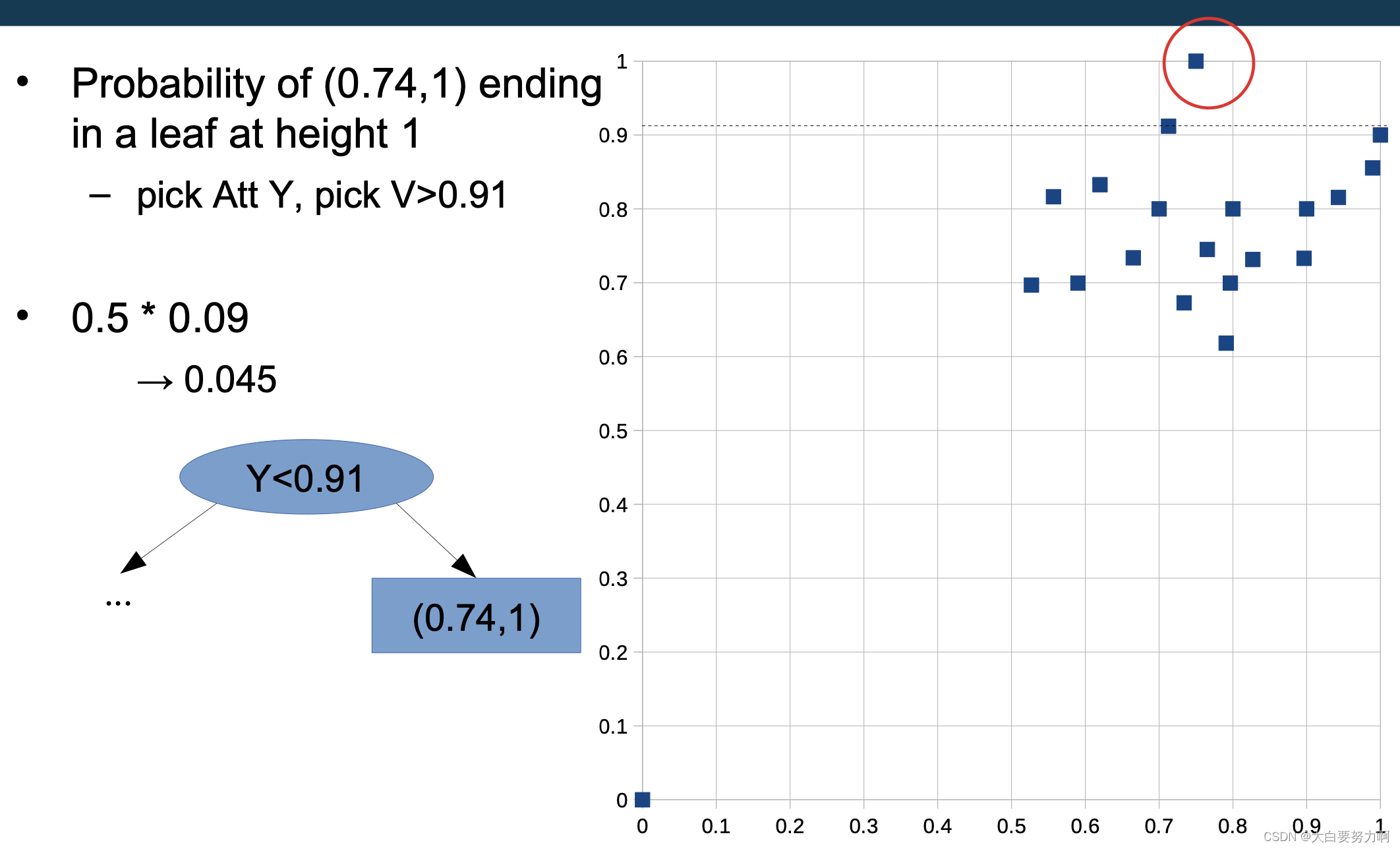
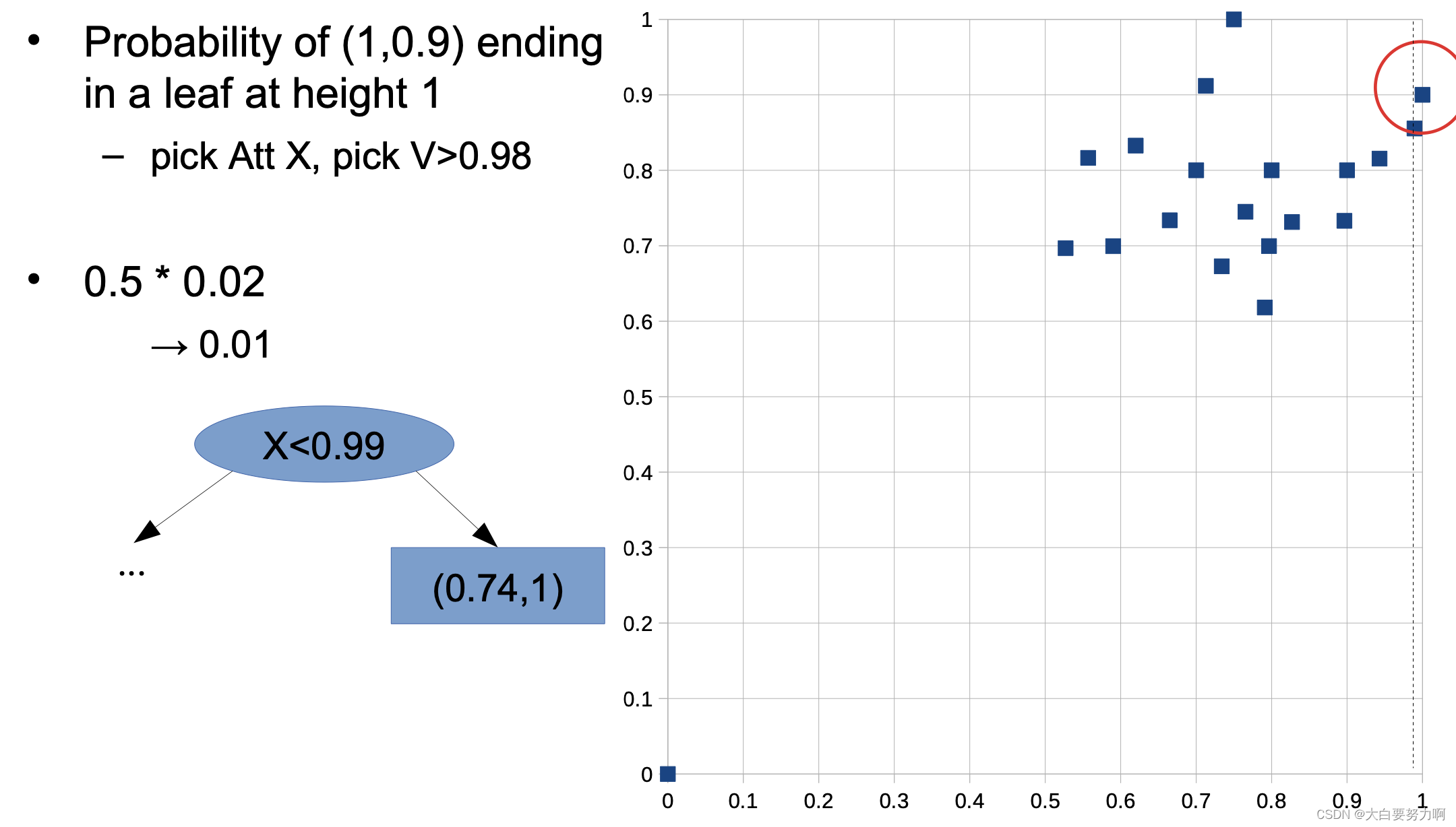
Idea: path to outliers in a tree is shorter than path to normal points; across a set of random trees, average path length is an outlier score

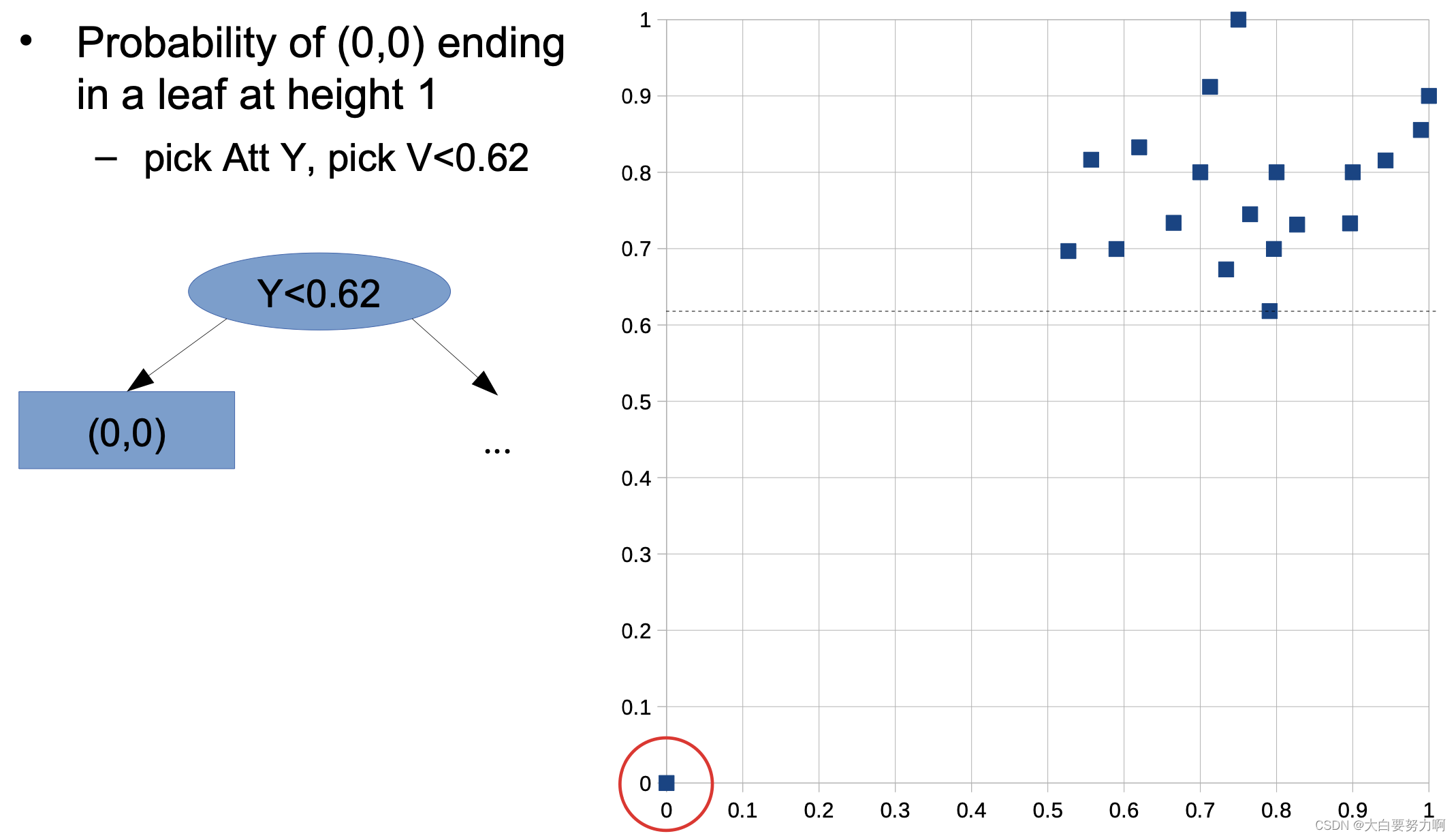
Training a single isolation tree
for each leaf node w/ more than one data point
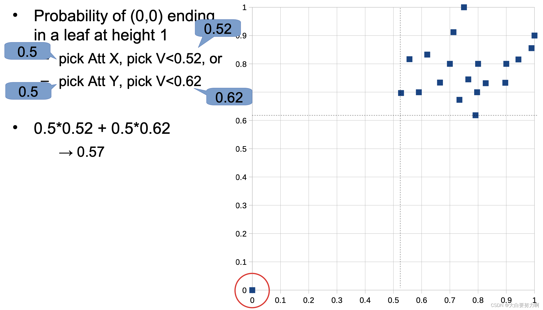
-> pick an attribute Att and a value V at random
-> create inner node with test Att < V (train isolation tree for each subtree)

Output
A tree with just one instance per node
Usually, an upper limit on height is used

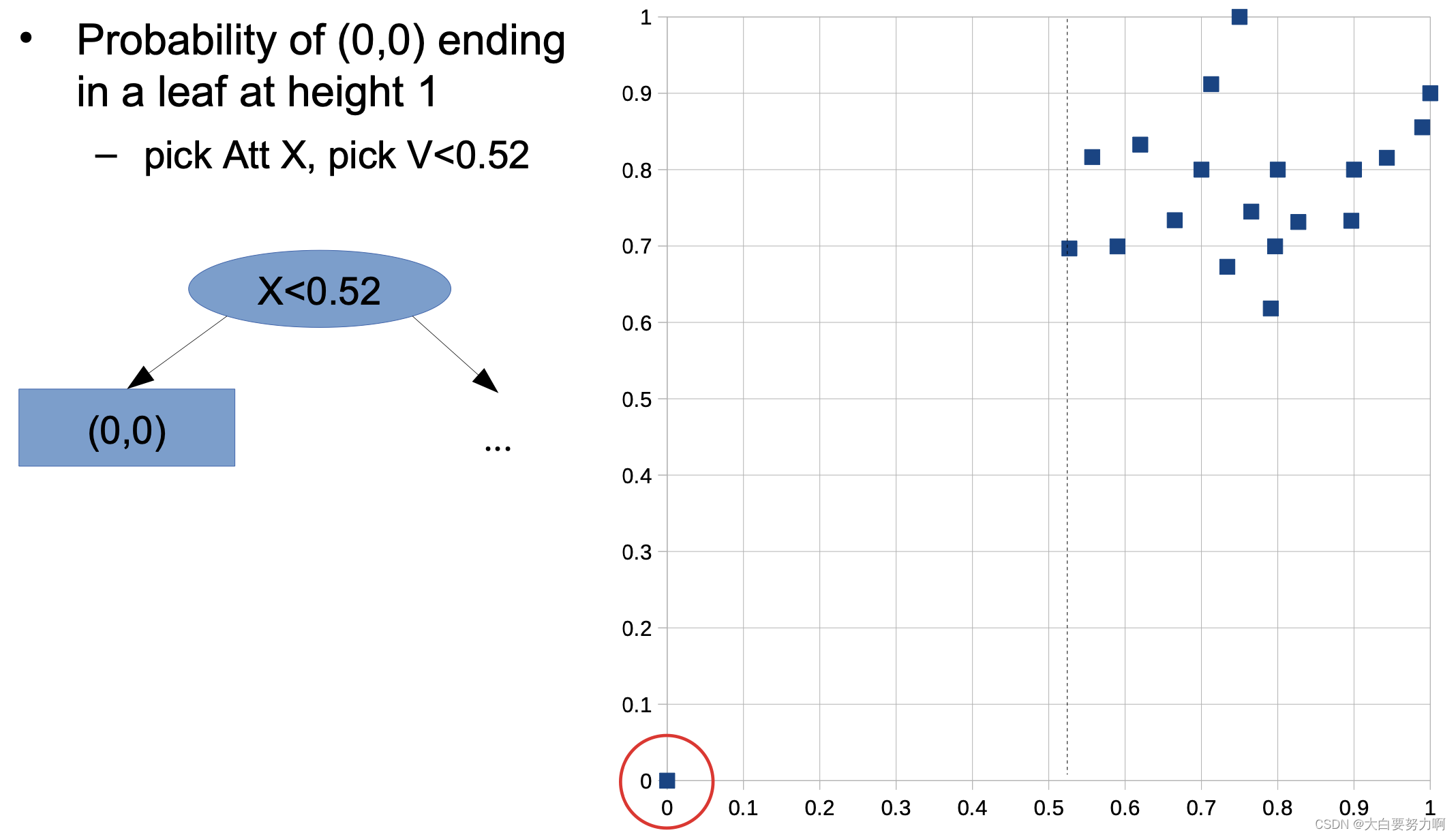
Probability of any other data point ending in a leaf at height 1 -this is not possible! at least two tests are necessary.

High-Dimensional Spaces
A large number of attributes may cause problems: many anomaly detection approaches use distance measures. Those get problematic for very high-dimensional spaces. Meaningless attributes obscure the distances

Practical Hint:
perform dimensionality reduction first, i.e., feature subset selection, PCA
note: anomaly detection is unsupervised. Thus, supervised selection (like forward/backward selection) does not work

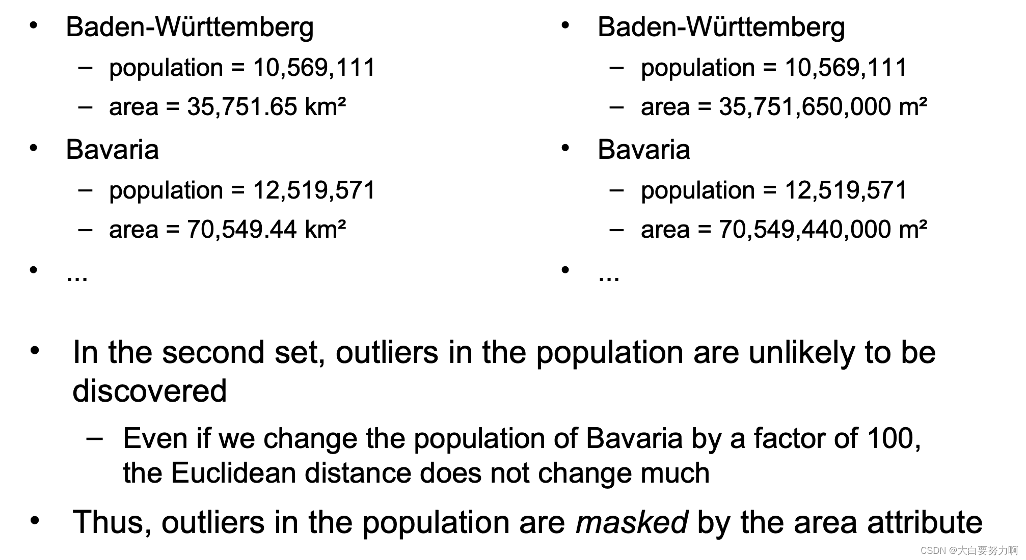
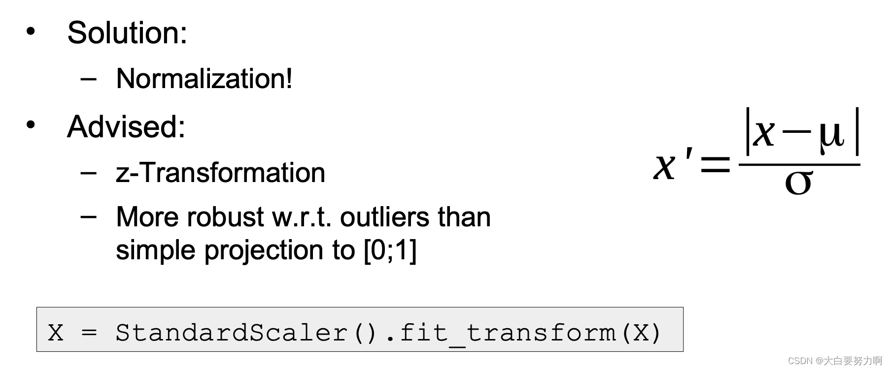
Attributes may have different scales. Hence, different attributes may have different contributions to outlier scores.

5.6 Evaluation Measures

Anomaly Detection is an unsupervised task
Evaluation: usually on a labeled subsample – Note: no splitting into training and test data!

Evaluation Measures

• F-measure on outliers
• Area under ROC curve
• Plots false positives against true positives

5.7 Semi-Supervised Anomaly Detection

All approaches discussed so far are unsupervised – they run fully automatic without human intelligence

Semi-Supervised Anomaly Detection
Experts manually label some data points as being outliers or not → anomaly detection becomes similar to a classification task
The class label being outlier/non-outlier

Challenges:

• Outliers are scarce → unbalanced dataset
• Outliers are not a class

Example: Outlier Detection in DBpedia
DBpedia is based on heuristic extraction
Several things can go wrong: wrong data in Wikipedia, unexpected number/date formats, errors in the extraction code, …
Challenge: Wikipedia is made for humans, not machines; Input format in Wikipedia is not constrained

Preprocessing: split data for different types
height is used for persons or buildings
population is used for villages, cities, countries, and continents
…

Separate into single distributions – makes anomaly detection better
Result
errors are identified at ~90% precision
systematic errors in the extraction code can be found

Typical error sources
unit conversions gone wrong (e.g., imperial/metric)
misinterpretation of numbers

Example: population: 28,322,006
e.g., village Semaphore in Australia (all of Australia: 23,379,555!)
a clear outlier among villages

Errors vs. Natural Outliers
Hard task for a machine
e.g., a 7.4m high vehicle
e.g., an adult person 58cm high

5.8 Summary