九、boosting和Adaboost学习

一、Boosting方法的基本思路

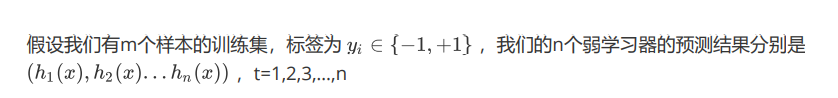
所谓 Boosting ，就是将弱分离器 f_i(x) 组合起来形成强分类器 F(x) 的一种方法。

Boosting的提出与发展离不开Valiant和 Kearns的努力，历史上正是Valiant和 Kearns提出了"强可学习"和"弱可学习"的概念。那什么是"强可学习"和"弱可学习"呢？在概率近似正确PAC学习的框架下：

• 弱学习：识别错误率小于1/2（即准确率仅比随机猜测略高的学习算法）

• 强学习：识别准确率很高并能在多项式时间内完成的学习算法

 非常有趣的是，在PAC 学习的框架下，强可学习和弱可学习是等价的，也就是说一个概念是强可学习的充分必要条件是这个概念是弱可学习的。

bosting就是从弱学习算法出发，反复学习，得到一系列弱分类器(又称为基本分类器)，然后通过一定的形式去组合这些弱分类器构成一个强分类器。
大多数的Boosting方法都是通过改变训练数据集的概率分布(训练数据不同样本的权值)，针对不同概率分布的数据调用弱分类算法学习一系列的弱分类器。

对于Boosting方法来说，有两个问题需要给出答案：

• 第一个是每一轮学习应该如何改变数据的概率分布。
• 第二个是如何将各个弱分类器组合起来。
  关于这两个问题，不同的Boosting算法会有不同的答案，我们接下来介绍一种最经典的Boosting算法----Adaboost，我们需要理解Adaboost是怎么处理这两个问题以及为什么这么处理的。
  

二、bagging和boosting区别

比较项	bagging	Boosting
样本选择	Bagging 算法是有放回的随机抽样；	Boosting 算法每一轮训练集不变，只是训练集中的每个样例在分类器中的权重发生变化，而权重根据上一轮分类结果进行调整；
样例权重	Bagging 使用随机抽样，样例权重一致；	Boosting 则根据错误率不断调整样例权重值，错误率越大权重越大；
预测函数	Bagging 所有预测模型的权重相等；	Boosting 算法对于误差小的分类器具有更大的权重；
并行计算	Bagging 算法可以并行生成各个基模型	Boosting 理论上只能顺序生产，因为每一个模型都需要上一个模型的结果；
减少项	Bagging 是减少模型的 Variance（方差）	Boosting 是减少模型的 Bias（偏差）
分类器	Bagging 里每个模型都是强分类器，因为降低的是方差，方差过高需要降低是过拟合；	Boosting 里每个分类模型都是弱分类器，因为降低的是偏差，偏度过高是欠拟合

三、Adaboost的基本原理

3.1 概述

对于Adaboost来说，解决上述的两个问题的方式是：

1. 提高那些被前一轮分类器错误分类的样本的权重，而降低那些被正确分类的样本的权重。
2. 各个弱分类器的组合是通过采取加权多数表决的方式，具体来说，加大分类错误率低的弱分类器的权重，因为这些分类器能更好地完成分类任务，而减小分类错误率较大的弱分类器的权重，使其在表决中起较小的作用。现在，我们来具体介绍Adaboost算法：(参考李航老师的《统计学习方法》)

3.2 算法步骤

• 1、计算样本的权重
  

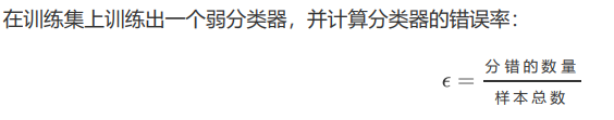
• 2、计算错误率
  

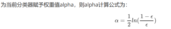
• 3、计算弱分类器的权重
  

• 4、调整权重值
  

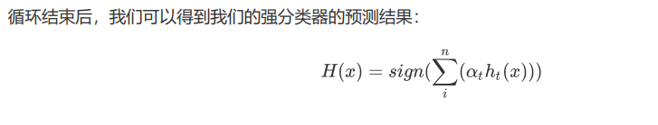
• 5、最终强分类器的结果
  

3.3 adaboost实例

训练数据如下表，假设基本分类器的形式是一个分割$x<v$或$x>v$表示，阈值v由该基本分类器在训练数据集上分类错误率$e_m$最低确定。
$$\begin{array}{ccccccccccc}\text{ 序号 }& 1& 2& 3& 4& 5& 6& 7& 8& 9& 10\\ x& 0& 1& 2& 3& 4& 5& 6& 7& 8& 9\\ y& 1& 1& 1& -1& -1& -1& 1& 1& 1& -1\end{array}$$
解：
初始化样本权值分布
$$\begin{array}{rl}{D}_1& =\left(w_{11},w_{12},\cdots ,w_{110}\right)\\ w_{1i}& =0.1,i=1,2,\cdots ,10\end{array}$$
对m=1:

• 在权值分布$D_1$的训练数据集上，遍历每个结点并计算分类误差率$e_m$，阈值取v=2.5时分类误差率最低，那么基本分类器为：
  $$G_1(x)=\{\begin{array}{ll}1,& x<2.5\\ -1,& x>2.5\end{array}$$
• $G_1(x)$在训练数据集上的误差率为$e_1=P\left(G_1\left(x_i\right)\ne y_i\right)=0.3$。
• 计算$G_1(x)$的系数：${\alpha }_1=\frac{1}{2}\log \frac{1-e_1}{e_1}=0.4236$
• 更新训练数据的权值分布：
  $$\begin{array}{rl}{D}_2=& \left(w_{21},\cdots ,w_{2i},\cdots ,w_{210}\right)\\ w_{2i}=& \frac{w_{1i}}{Z_1}\exp \left(-{\alpha }_1{y}_i{G}_1\left(x_i\right)\right),i=1,2,\cdots ,10\\ D_2=& (0.07143,0.07143,0.07143,0.07143,0.07143,0.07143,\\ & 0.16667,0.16667,0.16667,0.07143)\\ f_1(x)& =0.4236G_1(x)\end{array}$$

对于m=2：

• 在权值分布$D_2$的训练数据集上，遍历每个结点并计算分类误差率$e_m$，阈值取v=8.5时分类误差率最低，那么基本分类器为：
  $$G_2(x)=\{\begin{array}{ll}1,& x<8.5\\ -1,& x>8.5\end{array}$$
• $G_2(x)$在训练数据集上的误差率为$e_2=0.2143$
• 计算$G_2(x)$的系数：${\alpha }_2=0.6496$
• 更新训练数据的权值分布：
  $$\begin{array}{rl}{D}_3=& (0.0455,0.0455,0.0455,0.1667,0.1667,0.1667\\ & 0.1060,0.1060,0.1060,0.0455)\\ f_2(x)& =0.4236G_1(x)+0.6496G_2(x)\end{array}$$

对m=3：

• 在权值分布$D_3$的训练数据集上，遍历每个结点并计算分类误差率$e_m$，阈值取v=5.5时分类误差率最低，那么基本分类器为：
  $$G_3(x)=\{\begin{array}{ll}1,& x>5.5\\ -1,& x<5.5\end{array}$$
• $G_3(x)$在训练数据集上的误差率为$e_3=0.1820$
• 计算$G_3(x)$的系数：${\alpha }_3=0.7514$
• 更新训练数据的权值分布：
  $$D_4=(0.125,0.125,0.125,0.102,0.102,0.102,0.065,0.065,0.065,0.125)$$

于是得到：$f_3(x)=0.4236G_1(x)+0.6496G_2(x)+0.7514G_3(x)$，分类器$\mathrm{sign}\left[f_3(x)\right]$在训练数据集上的误分类点的个数为0。
于是得到最终分类器为：$G(x)=\mathrm{sign}\left[f_3(x)\right]=\mathrm{sign}\left[0.4236G_1(x)+0.6496G_2(x)+0.7514G_3(x)\right]$

四、使用sklearn对Adaboost算法进行建模

# 引入数据科学相关工具包：
import numpy as np
import pandas as pd 
import matplotlib.pyplot as plt
plt.style.use("ggplot")
%matplotlib inline
import seaborn as sns

# 加载训练数据：         
wine = pd.read_csv("https://archive.ics.uci.edu/ml/machine-learning-databases/wine/wine.data",header=None)
wine.columns = ['Class label', 'Alcohol', 'Malic acid', 'Ash', 'Alcalinity of ash','Magnesium',
                'Total phenols','Flavanoids', 'Nonflavanoid phenols', 
                'Proanthocyanins','Color intensity', 'Hue','OD280/OD315 of diluted wines','Proline']

# 数据查看：
print("Class labels",np.unique(wine["Class label"]))
wine.head()

Class labels [1 2 3]

	Class label	Alcohol	Malic acid	Ash	Alcalinity of ash	Magnesium	Total phenols	Flavanoids	Nonflavanoid phenols	Proanthocyanins	Color intensity	Hue	OD280/OD315 of diluted wines	Proline
0	1	14.23	1.71	2.43	15.6	127	2.80	3.06	0.28	2.29	5.64	1.04	3.92	1065
1	1	13.20	1.78	2.14	11.2	100	2.65	2.76	0.26	1.28	4.38	1.05	3.40	1050
2	1	13.16	2.36	2.67	18.6	101	2.80	3.24	0.30	2.81	5.68	1.03	3.17	1185
3	1	14.37	1.95	2.50	16.8	113	3.85	3.49	0.24	2.18	7.80	0.86	3.45	1480
4	1	13.24	2.59	2.87	21.0	118	2.80	2.69	0.39	1.82	4.32	1.04	2.93	735

下面对数据做简单解读：

• Class label：分类标签
• Alcohol：酒精
• Malic acid：苹果酸
• Ash：灰
• Alcalinity of ash：灰的碱度
• Magnesium：镁
• Total phenols：总酚
• Flavanoids：黄酮类化合物
• Nonflavanoid phenols：非黄烷类酚类
• Proanthocyanins：原花青素
• Color intensity：色彩强度
• Hue：色调
• OD280/OD315 of diluted wines：稀释酒OD280 OD350
• Proline：脯氨酸

# 数据预处理
# 仅仅考虑2，3类葡萄酒，去除1类
wine = wine[wine['Class label'] != 1]
y = wine['Class label'].values
X = wine[['Alcohol','OD280/OD315 of diluted wines']].values

# 将分类标签变成二进制编码：
from sklearn.preprocessing import LabelEncoder
le = LabelEncoder()
y = le.fit_transform(y)

# 按8：2分割训练集和测试集
from sklearn.model_selection import train_test_split
# stratify参数代表了按照y的类别等比例抽样
X_train,X_test,y_train,y_test = train_test_split(X,y,test_size=0.2,random_state=1,stratify=y)  

# 使用单一决策树建模
from sklearn.tree import DecisionTreeClassifier
tree = DecisionTreeClassifier(criterion='entropy',random_state=1,max_depth=1)
from sklearn.metrics import accuracy_score
tree = tree.fit(X_train,y_train)
y_train_pred = tree.predict(X_train)
y_test_pred = tree.predict(X_test)
tree_train = accuracy_score(y_train,y_train_pred)
tree_test = accuracy_score(y_test,y_test_pred)
print('Decision tree train/test accuracies %.3f/%.3f' % (tree_train,tree_test))

Decision tree train/test accuracies 0.916/0.875

# 使用sklearn实现Adaboost(基分类器为决策树)
'''
AdaBoostClassifier相关参数：
base_estimator：基本分类器，默认为DecisionTreeClassifier(max_depth=1)
n_estimators：终止迭代的次数
learning_rate：学习率
algorithm：训练的相关算法，{'SAMME'，'SAMME.R'}，默认='SAMME.R'
random_state：随机种子
'''
from sklearn.ensemble import AdaBoostClassifier
ada = AdaBoostClassifier(base_estimator=tree,n_estimators=500,learning_rate=0.1,random_state=1)
ada = ada.fit(X_train,y_train)
y_train_pred = ada.predict(X_train)
y_test_pred = ada.predict(X_test)
ada_train = accuracy_score(y_train,y_train_pred)
ada_test = accuracy_score(y_test,y_test_pred)
print('Adaboost train/test accuracies %.3f/%.3f' % (ada_train,ada_test))

Adaboost train/test accuracies 1.000/0.917

结果分析
单层决策树似乎对训练数据欠拟合，而Adaboost模型正确地预测了训练数据的所有分类标签，而且与单层决策树相比，Adaboost的测试性能也略有提高。然而，为什么模型在训练集和测试集的性能相差这么大呢？我们使用图像来简单说明下这个道理！

# 画出单层决策树与Adaboost的决策边界：
x_min = X_train[:, 0].min() - 1
x_max = X_train[:, 0].max() + 1
y_min = X_train[:, 1].min() - 1
y_max = X_train[:, 1].max() + 1
xx, yy = np.meshgrid(np.arange(x_min, x_max, 0.1),np.arange(y_min, y_max, 0.1))
f, axarr = plt.subplots(nrows=1, ncols=2,sharex='col',sharey='row',figsize=(12, 6))
for idx, clf, tt in zip([0, 1],[tree, ada],['Decision tree', 'Adaboost']):
    clf.fit(X_train, y_train)
    Z = clf.predict(np.c_[xx.ravel(), yy.ravel()])
    Z = Z.reshape(xx.shape)
    axarr[idx].contourf(xx, yy, Z, alpha=0.3)
    axarr[idx].scatter(X_train[y_train==0, 0],X_train[y_train==0, 1],c='blue', marker='^')
    axarr[idx].scatter(X_train[y_train==1, 0],X_train[y_train==1, 1],c='red', marker='o')
    axarr[idx].set_title(tt)
axarr[0].set_ylabel('Alcohol', fontsize=12)
plt.tight_layout()
plt.text(0, -0.2,s='OD280/OD315 of diluted wines',ha='center',va='center',fontsize=12,transform=axarr[1].transAxes)
plt.show()

从上面的决策边界图可以看到：

Adaboost模型的决策边界比单层决策树的决策边界要复杂的多。也就是说，Adaboost试图用增加模型复杂度而降低偏差的方式去减少总误差，但是过程中引入了方差，可能出现过拟合，因此在训练集和测试集之间的性能存在较大的差距，这就简单地回答的刚刚问题。值的注意的是：与单个分类器相比，Adaboost等Boosting模型增加了计算的复杂度，在实践中需要仔细思考是否愿意为预测性能的相对改善而增加计算成本，而且Boosting方式无法做到现在流行的并行计算的方式进行训练，因为每一步迭代都要基于上一部的基本分类器。

五、总结

关于这一次的boosting学习，让我感受到集成学习的神奇，特别是在看了周志华老师的课之后，boosting的强大更加入我心了，特别的有意思，另外关于这次的学习我觉得不能够钻牛角尖，不然的话会越学越来的迷惑，当然能搞清楚，有所收获也是好的。感谢阅读。