主成分分析(PCA)与梯度上升

最新推荐文章于 2024-05-05 12:05:57 发布

德乌大青蛙

最新推荐文章于 2024-05-05 12:05:57 发布

阅读量356

点赞数

分类专栏：机器学习算法文章标签：机器学习

本文链接：https://blog.csdn.net/weixin_45137294/article/details/123996784

版权

机器学习算法专栏收录该内容

11 篇文章 9 订阅

订阅专栏

引言

主成分分析算法（PCA）主要用于数据降维，它的目标是通过某种线性投影，将高维的数据映射到低维的空间中，并期望在所投影的维度上数据的信息量最大，以此使用较少的数据维度，同时保留住较多的原数据点的特性。主成分分析法也能更方便的可视化数据以及对数据去噪。

主成分分析法原理

在这里插入图片描述

在一个2维空间中，样本有2个特征，如果对数据进行降维，降到1维，首先将样本点全部映射到x轴或者全部映射到y轴。当样本点映射到x轴或y轴时发现样本点之前的距离压缩较大，此时我们可以寻找出一条直线，样本点映射到这条直线上样本点之间的距离相距最大。主成分分析法就是寻找这样的一条直线，一般用方差来定义样本间的距离，方差越大代表样本间距离越大越小代表距离越近。方差表达式如下：
$Var(x)=\frac{1}{m}\sum_{i=1}^{m} {(x_i-\bar{x})^2}$

主成分分析步骤

1、将样本的均值归0，归0之样本在每一个维度的均值都为0，即 $\bar{x}=0，$ 此时 $Var(x)=\frac{1}{m}\sum_{i=1}^{m} {x_i^2}$ ， $x_i$ 为映射后的点，归0后样本空间如下：

2、求一个轴的方向 $w=(w_1,w_2)$ 使得所有样本点映射到 $w$ 上，使得方差 $Var(x)=\frac{1}{m}\sum_{i=1}^{m} {x_{pr}^2}$ 最大。由于 $x_{pr}$ 是一个向量，

$(X\cdot W)^2$
$(\ \mid\mid X \mid\mid \cdot \mid\mid W \mid\mid \cdot \cos \theta)^2$
当 $W$ 为单位向量时， $∣ ∣ W ∣ ∣ = 1$
$(\ \mid\mid X \mid\mid \cdot \mid\mid W \mid\mid \cdot \cos \theta)^2=(||X||\cdot \cos \theta)^2$
$X_{pr}||^2$
$Var(x)=\frac{1}{m}\sum_{i=1}^{m} {x_{pr}^2}=\frac{1}{m}\sum_{i=1}^{m} {(X \cdot W)^2}$

在这里插入图片描述
此时方差函数可以转换成如下公式，此时求方差最大值可以使用梯度上升法。
$Var(x)=\frac{1}{m}\sum_{i=1}^{m} {(X\cdot W)^2}$
$=\frac{1}{m}\sum_{i=1}^{m} {(X_1W_1+……+X_nW_n)^2}$
$=\frac{1}{m}\sum_{i=1}^{m} {(\sum_{j=1}^{n}{X_jW_j})^2}$

梯度上升法求解PCA问题

公式推导

求 $W$ ，使得 $=\frac{1}{m}\sum_{i=1}^{m} {(X_1^iW_1+……+X_n^iW_n)^2}$ 最大，对 $W$ 求导得：
在这里插入图片描述

python实现

import numpy as np
import matplotlib.pyplot as plt


def de_mean(x):
    return x - np.mean(x, axis=0)


def f(x, w):
    return np.sum((x.dot(w)) ** 2) / len(x)


def df(x, w):
    return 2 * x.T.dot(x.dot(w)) / len(x)


def deriction(w):
    return w / np.linalg.norm(w)


def gradient_ascent(x, w, alpha, n_iters=1e4, epslion=1e-8):
    cur_iter = 1
    while cur_iter < n_iters:
        last_w = w
        gradient = df(x, w)
        w = w + alpha * gradient
        w = deriction(w)
        if abs(f(x, w) - f(x, last_w)) < epslion:
            break

        cur_iter += 1
    return w


x = np.empty((100, 2))
x[:, 0] = np.random.normal(1, 100, size=100)
x[:, 1] = 0.45 * x[:, 0] + 4 + np.random.normal(0, 10, size=100)

x_mean = de_mean(x)
initial_w = np.random.random(x.shape[1])
w = gradient_ascent(x, initial_w, 0.01)

plt.scatter(x[:, 0], x[:, 1])
plt.plot([0, w[0] * 100], [0, w[1] * 100], color='r')
plt.show()

在这里插入图片描述

数据的前n个主成分

原理

样本点本身都是二维的坐标点，将它们映射到W轴之后，现在它们还不是一个一维的数据，只不过将这些坐标点相应的一个维度从原来的X轴和Y轴中其中的一个轴变成了W轴。相应的，它们还是二维的数据，它们还应该有另外的一个轴，当然这只是对二维数据来说。如果对于一个n维数据来说，对应的它还是应该有n个轴，只不过现在这n个轴通过 PCA 这种方法重新进行了排列，使得第一个轴保持了这些样本相应的方差是最大的，第二个轴次之，第三个轴再次之，依此类推。
PCA 方法本质上是从一组坐标系转移到另外一个坐标系这样的一个过程，由于之前求出了对于新的坐标系来说第一个轴所在的方向，那么下面的问题就是如何求出下一个轴所在的方向呢？由于已经求出第一主成分了，所以可以将数据进行改变，将数据在第一主成分的分量去掉。
在这里插入图片描述 $X^{\prime (i)}=X^{(i)}-X^{(i)}_{pr}$
$X^{(i)}_{pr}=||X^{(i)}_{pr}|| * W$
$||X^{(i)}_{pr}||=X^{(i)} \cdot W$
$\ \ X^{\prime (i)}=X^{(i)} -(X^{(i)} \cdot W)* W$

python实现

import numpy as np
import matplotlib.pyplot as plt


def de_mean(x):
    return x - np.mean(x, axis=0)


def f(x, w):
    return np.sum((x.dot(w)) ** 2) / len(x)


def df(x, w):
    return 2 * x.T.dot(x.dot(w)) / len(x)


def deriction(w):
    return w / np.linalg.norm(w)


def gradient_ascent( x, w, alpha, n_iters=1e4, epslion=1e-8):
    cur_iter = 1
    while cur_iter < n_iters:
        last_w = w
        gradient = df(x, w)
        w = w + alpha * gradient
        w = deriction(w)
        if abs(f(x, w) - f(x, last_w)) < epslion:
            break

        cur_iter += 1
    return w


x = np.empty((100, 2))
x[:, 0] = np.random.normal(1, 100, size=100)
x[:, 1] = 0.45 * x[:, 0] + 4 + np.random.normal(0, 10, size=100)

x_mean = de_mean(x)
initial_w = np.random.random(x.shape[1])
w = gradient_ascent(x, initial_w, 0.01)

x2 = np.empty((100, 2))

for i in range(len(x)):
    x2[i] = x[i] - x[i].dot(w) * w

plt.scatter(x2[:, 0], x2[:, 1])
plt.show()

第二主成分分布如图
在这里插入图片描述

import numpy as np

def de_mean(x):
    return x - np.mean(x, axis=0)

def f(x, w):
    return np.sum((x.dot(w)) ** 2) / len(x)

def df(x, w):
    return 2 * x.T.dot(x.dot(w)) / len(x)

def deriction(w):
    return w / np.linalg.norm(w)

def gradient_ascent(x, w, alpha, n_iters=1e4, epslion=1e-8):
    cur_iter = 1
    while cur_iter < n_iters:
        last_w = w
        gradient = df(x, w)
        w = w + alpha * gradient
        w = deriction(w)
        if abs(f(x, w) - f(x, last_w)) < epslion:
            break

        cur_iter += 1
    return w


def get_n_components(n, x):
    x_mean = de_mean(x)
    x_n = np.copy(x_mean)
    res = []

    for n_i in range(n):

        # 每次随机生成一个w
        initial_w = np.random.random(x.shape[1])
        # 求第n个轴w_n
        w = gradient_ascent(x_n, initial_w, 0.01)
        res.append(w)

        # 求第n个主成分
        for i in range(len(x)):
            x_n[i] = x_mean[i] - x_mean[i].dot(w) * w

    return res

x = np.empty((100, 2))
x[:, 0] = np.random.normal(1, 100, size=100)
x[:, 1] = 0.45 * x[:, 0] + 4 + np.random.normal(0, 10, size=100)

a = get_n_components(2, x)
c = a[0].dot(a[1])
print(c)

输出为1.0221073648564172e-07，接近于0可以看出w_1与w_2垂直

高维数据映射为低维数据

原理

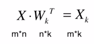
当一个n维数据要降为k（k<n）维数据时，只需要将样本数据点乘样本的前k个主成分矩阵 $W_k$ 的转置

在这里插入图片描述

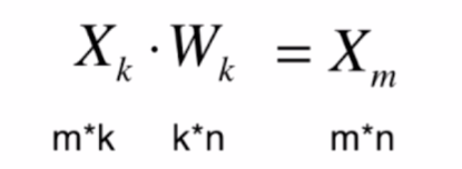
将数据恢复成n维数据公式，恢复之后不再是原来的数据

python实现

import numpy as np
import matplotlib.pyplot as plt

class PCA:
    def __init__(self,n_components):
        #初始化取前n个主成分
        self.n_components = n_components
        #主成分矩阵w
        self.componetnts_ = None

    def fit(self,x):
        def de_mean(x):
            return x - np.mean(x, axis=0)

        def f(x, w):
            return np.sum((x.dot(w)) ** 2) / len(x)

        def df(x, w):
            return 2 * x.T.dot(x.dot(w)) / len(x)

        def deriction(w):
            return w / np.linalg.norm(w)

        def gradient_ascent(x, w, alpha=0.01, n_iters=1e4, epslion=1e-8):
            cur_iter = 1
            while cur_iter < n_iters:
                last_w = w
                gradient = df(x, w)
                w = w + alpha * gradient
                w = deriction(w)
                if abs(f(x, w) - f(x, last_w)) < epslion:
                    break

                cur_iter += 1
            return w

        x_mean = de_mean(x)
        self.componetnts_ = np.empty(shape=(self.n_components,x.shape[1]))

        for i in range(self.n_components):

            # 每次随机生成一个w
            initial_w = np.random.random(x.shape[1])
            # 求第n个轴w_n
            w = gradient_ascent(x_mean, initial_w, 0.01)
            self.componetnts_[i] = w

            # 求第n个主成分
            x_mean = x_mean - x_mean.dot(w).reshape(-1,1) * w

    def transform(self,x):
        #将给定的X，映射到各个主成分分量中
        return x.dot(self.componetnts_.T)

    def inverse_transform(self,x):
        #将给定的X，反向映射回原来的特征空间
        return x.dot(self.componetnts_)

x = np.empty((100, 2))
x[:, 0] = np.random.normal(1, 100, size=100)
x[:, 1] = 0.45 * x[:, 0] + 4 + np.random.normal(0, 10, size=100)

pca = PCA(n_components=1)
pca.fit(x)
#映射到一维的数据
x2 = pca.transform(x - np.mean(x, axis=0))
#恢复到2维数据
x3 = pca.inverse_transform(x2)
print(x2)
plt.scatter(x3[:,0],x3[:,1],color='r')
plt.scatter(x[:,0],x[:,1],color='b')
plt.show()

可以看出恢复成2维的样本数据都分布在W轴上。
在这里插入图片描述

sklearn实现PCA算法

from sklearn.decomposition import PCA
from sklearn.datasets import load_digits
from sklearn.model_selection import train_test_split
from sklearn.neighbors import KNeighborsClassifier
import matplotlib.pyplot as plt

digits = load_digits()
x_data = digits.data
y_data = digits.target
x_train, x_test, y_train, y_test = train_test_split(x_data, y_data)

# pca初始化有两种方法：
# 1、取前n个主成分，n_components=2，
# 2、取百分之多少的数据方差，0-1
pca = PCA(n_components=x_train.shape[1]-1)
pca.fit(x_train, y_train)
x_train_reduction = pca.transform(x_train)
x_tes_reduction = pca.transform(x_test)
# 每个主成分能解释的数据方差，即每个主成分的重要程度
exp = pca.explained_variance_ratio_
print(exp.shape)

knn = KNeighborsClassifier()
knn.fit(x_train_reduction, y_train)
a = knn.score(x_tes_reduction, y_test)
print(a)

plt.plot([i for i in range(x_train.shape[1])],
         [sum(pca.explained_variance_ratio_[:i + 1]) for i in range(x_train.shape[1])])
plt.show()

横轴为前n个主成分，纵轴为前n个主成分对数据的解释度。
在这里插入图片描述

MNIST数据集实例

from sklearn.datasets import fetch_openml
from sklearn.neighbors import KNeighborsClassifier
from sklearn.decomposition import PCA

mnist = fetch_openml("mnist_784")

x_data = mnist.data
y_data = mnist.target

x_train_data = x_data[:60000]
x_test_data = x_data[60000:]
y_train_data = y_data[:60000]
y_test_data = y_data[60000:]

pca = PCA(0.95)
pca.fit(x_train_data)
x_train_transform = pca.transform(x_train_data)
x_test_transform = pca.transform(x_test_data)

knn = KNeighborsClassifier()
knn.fit(x_train_transform, y_train_data)
sec = knn.score(x_test_transform, y_test_data)

数据从784维降到了154维，识别准确率达98%以上。

PCA对数据降噪

PCA对数据降噪即对数据先降维处理，在将降维后数据恢复成原来的维度

from sklearn.datasets import load_digits
import matplotlib.pyplot as plt
from sklearn.decomposition import PCA


def plot_digits(x):
    # subplot_kw={'xticks': [], 'yticks': []} x轴y轴设为空
    fig, axes = plt.subplots(10, 10, figsize=(10, 10), subplot_kw={'xticks': [], 'yticks': []})
    for i, ax in enumerate(axes.flat):
        print(i)
        print(ax)
        ax.imshow(x[i].reshape(8, 8))

    plt.show()


digits = load_digits()
x_data = digits.data
y_data = digits.target

# 对数据加噪音
noisy_digits = x_data + np.random.normal(0, 4, size=x_data.shape)

pca = PCA(0.3)
pca.fit(x_data)
reduction = pca.transform(noisy_digits)
induction = pca.inverse_transform(reduction)

example_x1 = noisy_digits[:100]
example_x2 = induction[:100]

# plot_digits(example_x1)
plot_digits(example_x2)

降噪前
在这里插入图片描述
降噪后

德乌大青蛙

关注

0
点赞
踩
1

收藏

觉得还不错? 一键收藏
打赏
0
评论
主成分分析(PCA)与梯度上升

引言主成分分析算法（PCA）主要用于数据降维，它的目标是通过某种线性投影，将高维的数据映射到低维的空间中，并期望在所投影的维度上数据的信息量最大，以此使用较少的数据维度，同时保留住较多的原数据点的特性。主成分分析法也能更方便的可视化数据以及对数据去噪。主成分分析法原理在一个2维空间中，样本有2个特征，如果对数据进行降维，降到1维，首先将样本点全部映射到x轴或者全部映射到y轴。当样本点映射到x轴或y轴时发现样本点之前的距离压缩较大，此时我们可以寻找出一条直线，样本点映射到这条直线上样本点之间的距离相距
复制链接

扫一扫