Task 01：数学建模算法（规划）

线性规划

matlab中线性规划标准格式

c = [2; 3; -5];
a = [2, -5, 1; 1, 3, 1];
b = [10; 12];
aeq = [1, 1, 1];
beq = 7;
x = linprog(-c, a, b, aeq, beq, zeros(3, 1))   
% zeros(3, 1)为三行一列零矩阵
value = c'*x

>> practice

Optimal solution found.

x =
    4.5000
    2.5000
         0
value =
   16.5000
>> 

c = [2; 3; 1];
a = [1, 4, 2; 3, 2, 0];
b = [8; 6];
x = linprog(c, -a, -b, [], [], zeros(3, 1))
value = c'*x

>> practice

Optimal solution found.

x =
    2.0000
         0
    3.0000
value =
    7.0000

运输问题（产销平衡）

指派问题

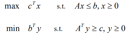
对偶问题

投资的收益和风险

整数规划

概论

分枝定界法

c = [40; 90];
a = [9, 7; 7, 20];
b = [56; 70];
x = linprog(-c, a, b, [], [], zeros(2, 1))
value = c'*x

>> test

Optimal solution found.

x =
    4.8092
    1.8168
value =
  355.8779        % 不管整数限定得到的最优解，不符合要求

此时z = 355.8779是最优目标函数值的上界，而x1 = 0，x2 = 0显然是问题的一个整数可行解，此时z = 0，是下界
因x1, x2均为非整数，不满足要求，任选一个进行分枝，设选x1进行分枝，把可行解分成两个子集，x1 ≤ 4.8092 = 4，x2 ≥ 4.8092 = 5

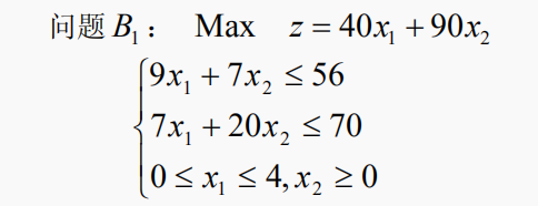
c = [40; 90];
a = [9, 7; 7, 20; 1, 0];
b = [56; 70; 4];
x = linprog(-c, a, b, [], [], zeros(2, 1))
value = c'*x

>> test

Optimal solution found.

x =
    4.0000
    2.1000
value =
   349

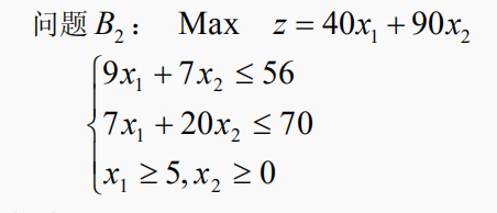
c = [40; 90];
a = [9, 7; 7, 20; -1, 0];
b = [56; 70; -5];
x = linprog(-c, a, b, [], [], zeros(2, 1))
value = c'*x

>> test

Optimal solution found.

x =
    5.0000
    1.5714
value =
  341.4286

分别对B1，B2再分枝

0 - 1型整数规划

蒙特卡洛法（随机取样法）

非线性规划

matlab解法

function f = fun1(x)              % 定义目标函数
f = sum(x.^2) + 8;

function [g, h] = fun2(x)         % 定义非线性约束条件
g = [-x(1) ^ 2 + x(2) - x(3) ^ 2
    x(1) + x(2) ^ 2 + x(3) ^ 3 - 20];
h = [-x(1) - x(2) ^ 2 + 2
    x(2) + 2 * x(3) ^ 2 - 3];

options = optimset('largescale', 'off');
[x, y] = fmincon('fun1', rand(3, 1), [], [], [], [], zeros(3, 1), [], ...
    'fun2', options)

>> example

Local minimum found that satisfies the constraints.

Optimization completed because the objective function is non-decreasing in 
feasible directions, to within the default value of the optimality tolerance,
and constraints are satisfied to within the default value of the constraint tolerance.

<stopping criteria details>

x =
    0.5522
    1.2033
    0.9478
y =
   10.6511