


通俗易懂地理解Gumbel Softmax
前言
我在学习《CLIP 改进工作串讲(上)【论文精读·42】》的过程中,听到朱老师讲到了GroupViT中用到了gumbel softmax(相关源代码),于是我带着好奇心试图想去了解gumbel softmax是什么,最后我把我的理解写成这篇文章,但是目前我在工作中还没用到gumbel softmax,所以如果有说得不对的地方,欢迎指正。
Gumbel-Softmax有什么用 ?
据我所知,gumbel softmax允许模型中有从离散的分布(比如类别分布categorical distribution)中采样的这个过程变得可微,从而允许反向传播时可以用梯度更新模型参数,所以这让gumbel softmax在深度学习的很多领域都有应用,比如分类分割任务、采样生成类任务AIGC、强化学习、语音识别、NAS等等。如果你是主动搜索到这篇文章的,那你对gumbel softamx的应用应该有自己的理解,如果跟我一样,暂时没用到的,也可以先学起来,说不定以后的算法能用上。
我们还是通过一个简单的例子来切入。假设我们有一个神经网络模型,模型中间某一层的输出是
nU(0, 1)采样出来的值,假设采样9个值,那就是[0.1, 0.2, 0.3, 0.4, 0.5, 0.6, 0.7, 0.8, 0.9],把这9个值作为y值代入gumbel 的CDF函数,求出x,这个x就是采样得到的值,这里使用下图的青色线演示:
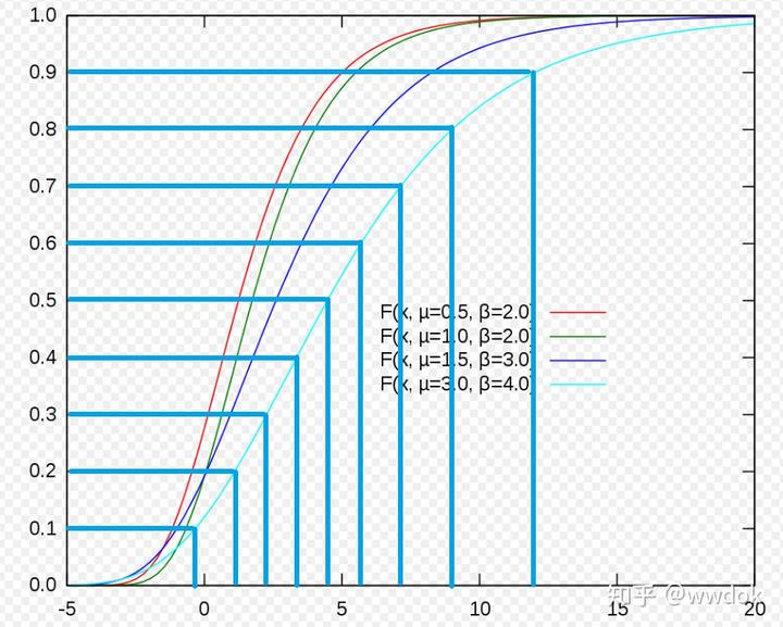

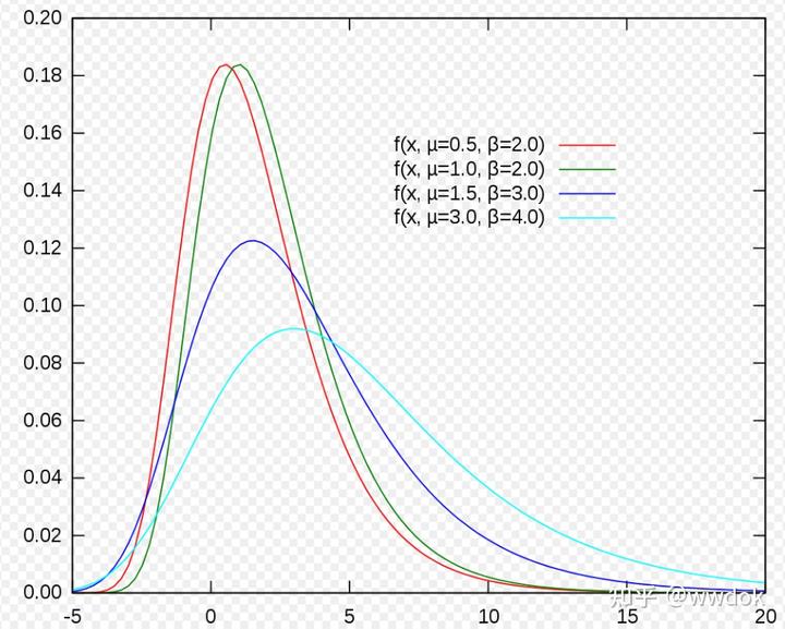
从上图我们可以感受到,采样值在x=3附近比较多,密度比较高,所以相应的它的概率密度函数(PDF,Probability Density Function)在x=3处是最大的,如下图所示:

写成代码的话,就是
import torch
gumbel分布的CDF函数的反函数
def inverse_gumbel_cdf(u, loc, beta):
return loc - scale * torch.log(-torch.log(u))
def gumbel_distribution_sampling(n, loc=0, scale=1):
u = torch.rand(n) #使用torch.rand生成均匀分布
g = inverse_gumbel_cdf(u, loc, scale)
return g
n = 10 # 采样个数
loc = 0 # gumbel分布的位置系数,类似于高斯分布的均值
scale = 1 # gumbel分布尺度系数,类似于高斯分布的标准差
samples = gumbel_distribution_sampling(n, loc, scale)
gumbel max trick公式里就用到了这个采样思想,即先用均匀分布采样出一个随机值,然后把这个值带入到gumbel分布的CDF函数的逆函数(inverse function,或者称为反函数)得到采样值。另外值得一说的是,gumbel max trick里使用的gumbel分布是标准gumbel分布,即 μ=0,β=1Z”就属于取极值的操作,所以它属于极值分布。在此之前,你可能想都不敢想,极值形成的分布竟然是有规律的,可的确就是有这么神奇的存在,这就是数学的魅力所在,但是要加个条件,就是极值是采样自某一个指数族的概率分布,比如高斯分布。
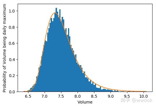
下面我们用一个例子和代码来验证一下这个极值分布的规律。假设你每天都会喝很多次水(比如100次),每次喝水的量服从正态分布N(μ,σ2)(其实也有点不合理,毕竟喝水的多少不能取为负值,不过无伤大雅能理解就好,假设均值为5),那么每天100次喝水里总会有一个最大值,这个最大值服从的分布就是Gumbel分布。
from scipy.optimize import curve_fit

import numpy as np

import matplotlib.pyplot as plt

mean_hunger = 5

samples_per_day = 100

n_days = 10000

samples = np.random.normal(loc=mean_hunger, scale=1.0, size=(n_days, samples_per_day))

daily_maxes = np.max(samples, axis=1)
# gumbel的通用PDF公式见维基百科
def gumbel_pdf(prob,loc,scale):
z = (prob-loc)/scale
return np.exp(-z-np.exp(-z))/scale
def plot_maxes(daily_maxes):
probs,bins,_ = plt.hist(daily_maxes,density=True,bins=100)
print(f“>> probs: {probs}“) # 每个bin的概率
print(f”>> bins: {bins}”) # 即横坐标的tick值
print(f“>> : {}“)
print(f”>> probs.shape: {probs.shape}”) # (100,)
print(f“==>> bins.shape: {bins.shape}”) # (101,)
plt.xlabel(‘Volume’)
plt.ylabel(‘Probability of Volume being daily maximum’)
<span class="c1"># 基于直方图,下面拟合出它的曲线。</span>
<span class="p">(</span><span class="n">fitted_loc</span><span class="p">,</span> <span class="n">fitted_scale</span><span class="p">),</span> <span class="n">_</span> <span class="o">=</span> <span class="n">curve_fit</span><span class="p">(</span><span class="n">gumbel_pdf</span><span class="p">,</span> <span class="n">bins</span><span class="p">[:</span><span class="o">-</span><span class="mi">1</span><span class="p">],</span><span class="n">probs</span><span class="p">)</span>
<span class="k">print</span><span class="p">(</span><span class="n">f</span><span class="s2">"==>> fitted_loc: {fitted_loc}"</span><span class="p">)</span>
<span class="k">print</span><span class="p">(</span><span class="n">f</span><span class="s2">"==>> fitted_scale: {fitted_scale}"</span><span class="p">)</span>
<span class="c1">#curve_fit用于曲线拟合,doc:https://docs.scipy.org/doc/scipy/reference/generated/scipy.optimize.curve_fit.html</span>
<span class="c1">#比如我们要拟合函数y=ax+b里的参数a和b,a和b确定了,这个函数就确定了,为了拟合这个函数,我们需要给curve_fit()提供待拟合函数的输入和输出样本</span>
<span class="c1">#所以curve_fit()的三个入参是:1.待拟合的函数(要求该函数的第一个入参是输入,后面的入参是要拟合的函数的参数)、2.样本输入、3.样本输出</span>
<span class="c1">#返回的是拟合好的参数,打包在元组里</span>
<span class="c1"># 其他教程:https://blog.csdn.net/guduruyu/article/details/70313176</span>
<span class="n">plt</span><span class="o">.</span><span class="n">plot</span><span class="p">(</span><span class="n">bins</span><span class="p">,</span> <span class="n">gumbel_pdf</span><span class="p">(</span><span class="n">bins</span><span class="p">,</span> <span class="n">fitted_loc</span><span class="p">,</span> <span class="n">fitted_scale</span><span class="p">))</span>
plt.figure()
plot_maxes(daily_maxes)

上面的例子中极值是采样自高斯分布,且是连续分布,那如果极值是采样自一个离散的类别分布呢,下面我们再用代码来验证一下。
如下代码定义了一个7类别的多项分布,每个类别的概率如下图
n_cats = 7

cats = np.arange(n_cats)

probs = np.random.randint(low=1, high=20, size=n_cats)

probs = probs / sum(probs)

logits = np.log(probs)

def plot_probs():

plt.bar(cats, probs)

plt.xlabel(“Category”)

plt.ylabel(“Probability”)

plt.figure()

plot_probs()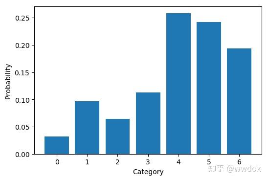

接下来我们将用代码演示为什么
z=argmaxi(log(πi)+gi)g_i得是gumbel分布,而不能是高斯分布或均匀分布
def sample_gumbel(logits):

noise = np.random.gumbel(size=len(logits))

sample = np.argmax(logits+noise)

return sample

gumbel_samples = [sample_gumbel(logits) for _ in range(n_samples)]
def sample_uniform(logits):
noise = np.random.uniform(size=len(logits))
sample = np.argmax(logits+noise)
return sample
uniform_samples = [sample_uniform(logits) for _ in range(n_samples)]
def sample_normal(logits):
noise = np.random.normal(size=len(logits))
sample = np.argmax(logits+noise)
return sample
normal_samples = [sample_normal(logits) for _ in range(n_samples)]
plt.figure(figsize=(10,4))
plt.subplot(1,4,1)
plot_probs()
plt.subplot(1,4,2)
gumbel_estd_probs = plot_estimated_probs(gumbel_samples,'Gumbel ')
plt.subplot(1,4,3)
normal_estd_probs = plot_estimated_probs(normal_samples,'Normal ')
plt.subplot(1,4,4)
uniform_estd_probs = plot_estimated_probs(uniform_samples,'Uniform ')
plt.tight_layout()
print(‘Original probabilities:\t\t’,end=‘’)
print_probs(probs)
print(‘Gumbel Estimated probabilities:\t’,end=‘’)
print_probs(gumbel_estd_probs)
print(‘Normal Estimated probabilities:\t’,end=‘’)
print_probs(normal_estd_probs)
print(‘Uniform Estimated probabilities:’,end=‘’)
print_probs(uniform_estd_probs)
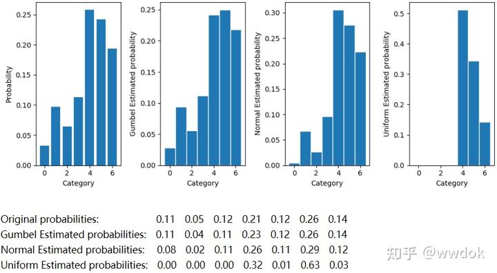

可以看到,只有加的噪声是gumbel分布,最后的概率分布才跟原来的分布差不多,加高斯分布和均匀分布的噪声的概率分布跟原来的概率分布明显差别很大。由此可见,
argmaxi(log(pi)+gi)p_{\tau}\left(v_{i}{\prime}\right)=\frac{e{v_{i}^{\prime} / \tau}}{\sum_{j=1}^{n} e{v_{j}{\prime} / \tau}}
pytorch相关函数说明
pytorch 提供的torch.nn.functional.gumbel_softmax api:https://pytorch.org/docs/stable/generated/torch.nn.functional.gumbel_softmax.html#torch.nn.functional.gumbel_softmax
视频讲解:《Gumbel Softmax补充说明》
实现的源代码:https://pytorch.org/docs/stable/modules/torch/nn/functional.html#gumbel_softmax
我这里对实现的源代码做一些说明:
# torch.nn.functional.gumbel_softmax的实现源码:
gumbels = (
-torch.empty_like(logits, memory_format=torch.legacy_contiguous_format).exponential().log()
) # ~Gumbel(0,1)
gumbels = (logits + gumbels) / tau # ~Gumbel(logits,tau)
y_soft = gumbels.softmax(dim)
<span class="k">if</span> <span class="n">hard</span><span class="p">:</span>
<span class="c1"># Straight through.</span>
<span class="n">index</span> <span class="o">=</span> <span class="n">y_soft</span><span class="o">.</span><span class="n">max</span><span class="p">(</span><span class="n">dim</span><span class="p">,</span> <span class="n">keepdim</span><span class="o">=</span><span class="bp">True</span><span class="p">)[</span><span class="mi">1</span><span class="p">]</span>
<span class="n">y_hard</span> <span class="o">=</span> <span class="n">torch</span><span class="o">.</span><span class="n">zeros_like</span><span class="p">(</span><span class="n">logits</span><span class="p">,</span> <span class="n">memory_format</span><span class="o">=</span><span class="n">torch</span><span class="o">.</span><span class="n">legacy_contiguous_format</span><span class="p">)</span><span class="o">.</span><span class="n">scatter_</span><span class="p">(</span><span class="n">dim</span><span class="p">,</span> <span class="n">index</span><span class="p">,</span> <span class="mf">1.0</span><span class="p">)</span>
<span class="n">ret</span> <span class="o">=</span> <span class="n">y_hard</span> <span class="o">-</span> <span class="n">y_soft</span><span class="o">.</span><span class="n">detach</span><span class="p">()</span> <span class="o">+</span> <span class="n">y_soft</span>
<span class="k">else</span><span class="p">:</span>
<span class="c1"># Reparametrization trick.</span>
<span class="n">ret</span> <span class="o">=</span> <span class="n">y_soft</span>
<span class="k">return</span> <span class="n">ret</span></code></pre></div><p data-pid="z3crAWAd">说明:</p><ol><li data-pid="idxuufP_">代码中的logits已经经过了log()处理,相当于公式里的<span class="ztext-math" data-eeimg="1" data-tex="log(p_i)"><span></span><span><span class="MathJax_Preview" style="color: inherit;"></span><span class="MathJax_SVG" id="MathJax-Element-53-Frame" tabindex="0" style="font-size: 100%; display: inline-block; position: relative;" data-mathml="<math xmlns="http://www.w3.org/1998/Math/MathML"><mi>l</mi><mi>o</mi><mi>g</mi><mo stretchy="false">(</mo><msub><mi>p</mi><mi>i</mi></msub><mo stretchy="false">)</mo></math>" role="presentation"><svg xmlns:xlink="http://www.w3.org/1999/xlink" width="6.715ex" height="2.789ex" viewBox="0 -849.8 2891.3 1200.9" role="img" focusable="false" aria-hidden="true" style="vertical-align: -0.815ex;"><g stroke="currentColor" fill="currentColor" stroke-width="0" transform="matrix(1 0 0 -1 0 0)"><use xlink:href="#MJMATHI-6C" x="0" y="0"></use><use xlink:href="#MJMATHI-6F" x="298" y="0"></use><use xlink:href="#MJMATHI-67" x="784" y="0"></use><use xlink:href="#MJMAIN-28" x="1264" y="0"></use><g transform="translate(1654,0)"><use xlink:href="#MJMATHI-70" x="0" y="0"></use><use transform="scale(0.707)" xlink:href="#MJMATHI-69" x="712" y="-213"></use></g><use xlink:href="#MJMAIN-29" x="2501" y="0"></use></g></svg><span class="MJX_Assistive_MathML" role="presentation"><math xmlns="http://www.w3.org/1998/Math/MathML"><mi>l</mi><mi>o</mi><mi>g</mi><mo stretchy="false">(</mo><msub><mi>p</mi><mi>i</mi></msub><mo stretchy="false">)</mo></math></span></span><script type="math/tex;mode=inline" id="MathJax-Element-53">log(p_i)</script><span class="tex2jax_ignore math-holder">log(p_i)</span></span></span></li></ol><p data-pid="gqp8BHS0">2. 在计算gumbels时,源码里使用了exponential_(),<a href="https://link.zhihu.com/?target=https%3A//pytorch.org/docs/stable/generated/torch.Tensor.exponential_.html" class=" wrap external" target="_blank" rel="nofollow noreferrer" data-za-detail-view-id="1043">它的文档</a>里说了,这代表的是从指数分布<span class="ztext-math" data-eeimg="1" data-tex="\lambda e^{-\lambda x}(\lambda=1)"><span></span><span><span class="MathJax_Preview" style="color: inherit;"></span><span class="MathJax_SVG" id="MathJax-Element-54-Frame" tabindex="0" style="font-size: 100%; display: inline-block; position: relative;" data-mathml="<math xmlns="http://www.w3.org/1998/Math/MathML"><mi>&#x03BB;</mi><msup><mi>e</mi><mrow class="MJX-TeXAtom-ORD"><mo>&#x2212;</mo><mi>&#x03BB;</mi><mi>x</mi></mrow></msup><mo stretchy="false">(</mo><mi>&#x03BB;</mi><mo>=</mo><mn>1</mn><mo stretchy="false">)</mo></math>" role="presentation"><svg xmlns:xlink="http://www.w3.org/1999/xlink" width="13.273ex" height="3.021ex" viewBox="0 -949.6 5715 1300.6" role="img" focusable="false" aria-hidden="true" style="vertical-align: -0.815ex;"><g stroke="currentColor" fill="currentColor" stroke-width="0" transform="matrix(1 0 0 -1 0 0)"><use xlink:href="#MJMATHI-3BB" x="0" y="0"></use><g transform="translate(583,0)"><use xlink:href="#MJMATHI-65" x="0" y="0"></use><g transform="translate(466,362)"><use transform="scale(0.707)" xlink:href="#MJMAIN-2212" x="0" y="0"></use><use transform="scale(0.707)" xlink:href="#MJMATHI-3BB" x="778" y="0"></use><use transform="scale(0.707)" xlink:href="#MJMATHI-78" x="1362" y="0"></use></g></g><use xlink:href="#MJMAIN-28" x="2517" y="0"></use><use xlink:href="#MJMATHI-3BB" x="2907" y="0"></use><use xlink:href="#MJMAIN-3D" x="3768" y="0"></use><use xlink:href="#MJMAIN-31" x="4824" y="0"></use><use xlink:href="#MJMAIN-29" x="5325" y="0"></use></g></svg><span class="MJX_Assistive_MathML" role="presentation"><math xmlns="http://www.w3.org/1998/Math/MathML"><mi>λ</mi><msup><mi>e</mi><mrow class="MJX-TeXAtom-ORD"><mo>−</mo><mi>λ</mi><mi>x</mi></mrow></msup><mo stretchy="false">(</mo><mi>λ</mi><mo>=</mo><mn>1</mn><mo stretchy="false">)</mo></math></span></span><script type="math/tex;mode=inline" id="MathJax-Element-54">\lambda e^{-\lambda x}(\lambda=1)</script><span class="tex2jax_ignore math-holder">\lambda e^{-\lambda x}(\lambda=1)</span></span></span>中采样,这跟我们前面公式里的<span class="ztext-math" data-eeimg="1" data-tex="g_i = -log(-log(u_i)), u_i \sim U(0,1)"><span></span><span><span class="MathJax_Preview" style="color: inherit;"></span><span class="MathJax_SVG" id="MathJax-Element-55-Frame" tabindex="0" style="font-size: 100%; display: inline-block; position: relative;" data-mathml="<math xmlns="http://www.w3.org/1998/Math/MathML"><msub><mi>g</mi><mi>i</mi></msub><mo>=</mo><mo>&#x2212;</mo><mi>l</mi><mi>o</mi><mi>g</mi><mo stretchy="false">(</mo><mo>&#x2212;</mo><mi>l</mi><mi>o</mi><mi>g</mi><mo stretchy="false">(</mo><msub><mi>u</mi><mi>i</mi></msub><mo stretchy="false">)</mo><mo stretchy="false">)</mo><mo>,</mo><msub><mi>u</mi><mi>i</mi></msub><mo>&#x223C;</mo><mi>U</mi><mo stretchy="false">(</mo><mn>0</mn><mo>,</mo><mn>1</mn><mo stretchy="false">)</mo></math>" role="presentation"><svg xmlns:xlink="http://www.w3.org/1999/xlink" width="33.458ex" height="2.789ex" viewBox="0 -849.8 14405.4 1200.9" role="img" focusable="false" aria-hidden="true" style="vertical-align: -0.815ex;"><g stroke="currentColor" fill="currentColor" stroke-width="0" transform="matrix(1 0 0 -1 0 0)"><use xlink:href="#MJMATHI-67" x="0" y="0"></use><use transform="scale(0.707)" xlink:href="#MJMATHI-69" x="675" y="-213"></use><use xlink:href="#MJMAIN-3D" x="1099" y="0"></use><use xlink:href="#MJMAIN-2212" x="2155" y="0"></use><use xlink:href="#MJMATHI-6C" x="2934" y="0"></use><use xlink:href="#MJMATHI-6F" x="3232" y="0"></use><use xlink:href="#MJMATHI-67" x="3718" y="0"></use><use xlink:href="#MJMAIN-28" x="4198" y="0"></use><use xlink:href="#MJMAIN-2212" x="4588" y="0"></use><use xlink:href="#MJMATHI-6C" x="5366" y="0"></use><use xlink:href="#MJMATHI-6F" x="5665" y="0"></use><use xlink:href="#MJMATHI-67" x="6150" y="0"></use><use xlink:href="#MJMAIN-28" x="6631" y="0"></use><g transform="translate(7020,0)"><use xlink:href="#MJMATHI-75" x="0" y="0"></use><use transform="scale(0.707)" xlink:href="#MJMATHI-69" x="809" y="-213"></use></g><use xlink:href="#MJMAIN-29" x="7937" y="0"></use><use xlink:href="#MJMAIN-29" x="8327" y="0"></use><use xlink:href="#MJMAIN-2C" x="8716" y="0"></use><g transform="translate(9161,0)"><use xlink:href="#MJMATHI-75" x="0" y="0"></use><use transform="scale(0.707)" xlink:href="#MJMATHI-69" x="809" y="-213"></use></g><use xlink:href="#MJMAIN-223C" x="10356" y="0"></use><use xlink:href="#MJMATHI-55" x="11412" y="0"></use><use xlink:href="#MJMAIN-28" x="12180" y="0"></use><use xlink:href="#MJMAIN-30" x="12569" y="0"></use><use xlink:href="#MJMAIN-2C" x="13070" y="0"></use><use xlink:href="#MJMAIN-31" x="13515" y="0"></use><use xlink:href="#MJMAIN-29" x="14015" y="0"></use></g></svg><span class="MJX_Assistive_MathML" role="presentation"><math xmlns="http://www.w3.org/1998/Math/MathML"><msub><mi>g</mi><mi>i</mi></msub><mo>=</mo><mo>−</mo><mi>l</mi><mi>o</mi><mi>g</mi><mo stretchy="false">(</mo><mo>−</mo><mi>l</mi><mi>o</mi><mi>g</mi><mo stretchy="false">(</mo><msub><mi>u</mi><mi>i</mi></msub><mo stretchy="false">)</mo><mo stretchy="false">)</mo><mo>,</mo><msub><mi>u</mi><mi>i</mi></msub><mo>∼</mo><mi>U</mi><mo stretchy="false">(</mo><mn>0</mn><mo>,</mo><mn>1</mn><mo stretchy="false">)</mo></math></span></span><script type="math/tex;mode=inline" id="MathJax-Element-55">g_i = -log(-log(u_i)), u_i \sim U(0,1)</script><span class="tex2jax_ignore math-holder">g_i = -log(-log(u_i)), u_i \sim U(0,1)</span></span></span>不太一样,它没有从均匀分布<span class="ztext-math" data-eeimg="1" data-tex="U(0,1)"><span></span><span><span class="MathJax_Preview" style="color: inherit;"></span><span class="MathJax_SVG" id="MathJax-Element-56-Frame" tabindex="0" style="font-size: 100%; display: inline-block; position: relative;" data-mathml="<math xmlns="http://www.w3.org/1998/Math/MathML"><mi>U</mi><mo stretchy="false">(</mo><mn>0</mn><mo>,</mo><mn>1</mn><mo stretchy="false">)</mo></math>" role="presentation"><svg xmlns:xlink="http://www.w3.org/1999/xlink" width="6.951ex" height="2.789ex" viewBox="0 -849.8 2992.7 1200.9" role="img" focusable="false" aria-hidden="true" style="vertical-align: -0.815ex;"><g stroke="currentColor" fill="currentColor" stroke-width="0" transform="matrix(1 0 0 -1 0 0)"><use xlink:href="#MJMATHI-55" x="0" y="0"></use><use xlink:href="#MJMAIN-28" x="767" y="0"></use><use xlink:href="#MJMAIN-30" x="1157" y="0"></use><use xlink:href="#MJMAIN-2C" x="1657" y="0"></use><use xlink:href="#MJMAIN-31" x="2102" y="0"></use><use xlink:href="#MJMAIN-29" x="2603" y="0"></use></g></svg><span class="MJX_Assistive_MathML" role="presentation"><math xmlns="http://www.w3.org/1998/Math/MathML"><mi>U</mi><mo stretchy="false">(</mo><mn>0</mn><mo>,</mo><mn>1</mn><mo stretchy="false">)</mo></math></span></span><script type="math/tex;mode=inline" id="MathJax-Element-56">U(0,1)</script><span class="tex2jax_ignore math-holder">U(0,1)</span></span></span>里采样,而是从指数分布<span class="ztext-math" data-eeimg="1" data-tex="e^{-x}"><span></span><span><span class="MathJax_Preview" style="color: inherit;"></span><span class="MathJax_SVG" id="MathJax-Element-57-Frame" tabindex="0" style="font-size: 100%; display: inline-block; position: relative;" data-mathml="<math xmlns="http://www.w3.org/1998/Math/MathML"><msup><mi>e</mi><mrow class="MJX-TeXAtom-ORD"><mo>&#x2212;</mo><mi>x</mi></mrow></msup></math>" role="presentation"><svg xmlns:xlink="http://www.w3.org/1999/xlink" width="3.535ex" height="2.21ex" viewBox="0 -849.8 1521.8 951.6" role="img" focusable="false" aria-hidden="true" style="vertical-align: -0.236ex;"><g stroke="currentColor" fill="currentColor" stroke-width="0" transform="matrix(1 0 0 -1 0 0)"><use xlink:href="#MJMATHI-65" x="0" y="0"></use><g transform="translate(466,362)"><use transform="scale(0.707)" xlink:href="#MJMAIN-2212" x="0" y="0"></use><use transform="scale(0.707)" xlink:href="#MJMATHI-78" x="778" y="0"></use></g></g></svg><span class="MJX_Assistive_MathML" role="presentation"><math xmlns="http://www.w3.org/1998/Math/MathML"><msup><mi>e</mi><mrow class="MJX-TeXAtom-ORD"><mo>−</mo><mi>x</mi></mrow></msup></math></span></span><script type="math/tex;mode=inline" id="MathJax-Element-57">e^{-x}</script><span class="tex2jax_ignore math-holder">e^{-x}</span></span></span>里采样,但是其实两者殊途同归,因为<span class="ztext-math" data-eeimg="1" data-tex="e^{-x}"><span></span><span><span class="MathJax_Preview" style="color: inherit;"></span><span class="MathJax_SVG" id="MathJax-Element-60-Frame" tabindex="0" style="font-size: 100%; display: inline-block; position: relative;" data-mathml="<math xmlns="http://www.w3.org/1998/Math/MathML"><msup><mi>e</mi><mrow class="MJX-TeXAtom-ORD"><mo>&#x2212;</mo><mi>x</mi></mrow></msup></math>" role="presentation"><svg xmlns:xlink="http://www.w3.org/1999/xlink" width="3.535ex" height="2.21ex" viewBox="0 -849.8 1521.8 951.6" role="img" focusable="false" aria-hidden="true" style="vertical-align: -0.236ex;"><g stroke="currentColor" fill="currentColor" stroke-width="0" transform="matrix(1 0 0 -1 0 0)"><use xlink:href="#MJMATHI-65" x="0" y="0"></use><g transform="translate(466,362)"><use transform="scale(0.707)" xlink:href="#MJMAIN-2212" x="0" y="0"></use><use transform="scale(0.707)" xlink:href="#MJMATHI-78" x="778" y="0"></use></g></g></svg><span class="MJX_Assistive_MathML" role="presentation"><math xmlns="http://www.w3.org/1998/Math/MathML"><msup><mi>e</mi><mrow class="MJX-TeXAtom-ORD"><mo>−</mo><mi>x</mi></mrow></msup></math></span></span><script type="math/tex;mode=inline" id="MathJax-Element-60">e^{-x}</script><span class="tex2jax_ignore math-holder">e^{-x}</span></span></span>的逆函数是<span class="ztext-math" data-eeimg="1" data-tex="-log(x)"><span></span><span><span class="MathJax_Preview" style="color: inherit;"></span><span class="MathJax_SVG" id="MathJax-Element-58-Frame" tabindex="0" style="font-size: 100%; display: inline-block; position: relative;" data-mathml="<math xmlns="http://www.w3.org/1998/Math/MathML"><mo>&#x2212;</mo><mi>l</mi><mi>o</mi><mi>g</mi><mo stretchy="false">(</mo><mi>x</mi><mo stretchy="false">)</mo></math>" role="presentation"><svg xmlns:xlink="http://www.w3.org/1999/xlink" width="7.884ex" height="2.789ex" viewBox="0 -849.8 3394.5 1200.9" role="img" focusable="false" aria-hidden="true" style="vertical-align: -0.815ex;"><g stroke="currentColor" fill="currentColor" stroke-width="0" transform="matrix(1 0 0 -1 0 0)"><use xlink:href="#MJMAIN-2212" x="0" y="0"></use><use xlink:href="#MJMATHI-6C" x="778" y="0"></use><use xlink:href="#MJMATHI-6F" x="1077" y="0"></use><use xlink:href="#MJMATHI-67" x="1562" y="0"></use><use xlink:href="#MJMAIN-28" x="2043" y="0"></use><use xlink:href="#MJMATHI-78" x="2432" y="0"></use><use xlink:href="#MJMAIN-29" x="3005" y="0"></use></g></svg><span class="MJX_Assistive_MathML" role="presentation"><math xmlns="http://www.w3.org/1998/Math/MathML"><mo>−</mo><mi>l</mi><mi>o</mi><mi>g</mi><mo stretchy="false">(</mo><mi>x</mi><mo stretchy="false">)</mo></math></span></span><script type="math/tex;mode=inline" id="MathJax-Element-58">-log(x)</script><span class="tex2jax_ignore math-holder">-log(x)</span></span></span>(其实代码里的log一般是ln),所以其实<span class="ztext-math" data-eeimg="1" data-tex="-log(u_i),u_i \sim U(0,1)"><span></span><span><span class="MathJax_Preview" style="color: inherit;"></span><span class="MathJax_SVG" id="MathJax-Element-59-Frame" tabindex="0" style="font-size: 100%; display: inline-block; position: relative;" data-mathml="<math xmlns="http://www.w3.org/1998/Math/MathML"><mo>&#x2212;</mo><mi>l</mi><mi>o</mi><mi>g</mi><mo stretchy="false">(</mo><msub><mi>u</mi><mi>i</mi></msub><mo stretchy="false">)</mo><mo>,</mo><msub><mi>u</mi><mi>i</mi></msub><mo>&#x223C;</mo><mi>U</mi><mo stretchy="false">(</mo><mn>0</mn><mo>,</mo><mn>1</mn><mo stretchy="false">)</mo></math>" role="presentation"><svg xmlns:xlink="http://www.w3.org/1999/xlink" width="21.896ex" height="2.789ex" viewBox="0 -849.8 9427.5 1200.9" role="img" focusable="false" aria-hidden="true" style="vertical-align: -0.815ex;"><g stroke="currentColor" fill="currentColor" stroke-width="0" transform="matrix(1 0 0 -1 0 0)"><use xlink:href="#MJMAIN-2212" x="0" y="0"></use><use xlink:href="#MJMATHI-6C" x="778" y="0"></use><use xlink:href="#MJMATHI-6F" x="1077" y="0"></use><use xlink:href="#MJMATHI-67" x="1562" y="0"></use><use xlink:href="#MJMAIN-28" x="2043" y="0"></use><g transform="translate(2432,0)"><use xlink:href="#MJMATHI-75" x="0" y="0"></use><use transform="scale(0.707)" xlink:href="#MJMATHI-69" x="809" y="-213"></use></g><use xlink:href="#MJMAIN-29" x="3349" y="0"></use><use xlink:href="#MJMAIN-2C" x="3738" y="0"></use><g transform="translate(4183,0)"><use xlink:href="#MJMATHI-75" x="0" y="0"></use><use transform="scale(0.707)" xlink:href="#MJMATHI-69" x="809" y="-213"></use></g><use xlink:href="#MJMAIN-223C" x="5378" y="0"></use><use xlink:href="#MJMATHI-55" x="6434" y="0"></use><use xlink:href="#MJMAIN-28" x="7202" y="0"></use><use xlink:href="#MJMAIN-30" x="7591" y="0"></use><use xlink:href="#MJMAIN-2C" x="8092" y="0"></use><use xlink:href="#MJMAIN-31" x="8537" y="0"></use><use xlink:href="#MJMAIN-29" x="9037" y="0"></use></g></svg><span class="MJX_Assistive_MathML" role="presentation"><math xmlns="http://www.w3.org/1998/Math/MathML"><mo>−</mo><mi>l</mi><mi>o</mi><mi>g</mi><mo stretchy="false">(</mo><msub><mi>u</mi><mi>i</mi></msub><mo stretchy="false">)</mo><mo>,</mo><msub><mi>u</mi><mi>i</mi></msub><mo>∼</mo><mi>U</mi><mo stretchy="false">(</mo><mn>0</mn><mo>,</mo><mn>1</mn><mo stretchy="false">)</mo></math></span></span><script type="math/tex;mode=inline" id="MathJax-Element-59">-log(u_i),u_i \sim U(0,1)</script><span class="tex2jax_ignore math-holder">-log(u_i),u_i \sim U(0,1)</span></span></span>代表的就是从指数分布<span class="ztext-math" data-eeimg="1" data-tex="e^{-x}"><span></span><span><span class="MathJax_Preview" style="color: inherit;"></span><span class="MathJax_SVG" id="MathJax-Element-61-Frame" tabindex="0" style="font-size: 100%; display: inline-block; position: relative;" data-mathml="<math xmlns="http://www.w3.org/1998/Math/MathML"><msup><mi>e</mi><mrow class="MJX-TeXAtom-ORD"><mo>&#x2212;</mo><mi>x</mi></mrow></msup></math>" role="presentation"><svg xmlns:xlink="http://www.w3.org/1999/xlink" width="3.535ex" height="2.21ex" viewBox="0 -849.8 1521.8 951.6" role="img" focusable="false" aria-hidden="true" style="vertical-align: -0.236ex;"><g stroke="currentColor" fill="currentColor" stroke-width="0" transform="matrix(1 0 0 -1 0 0)"><use xlink:href="#MJMATHI-65" x="0" y="0"></use><g transform="translate(466,362)"><use transform="scale(0.707)" xlink:href="#MJMAIN-2212" x="0" y="0"></use><use transform="scale(0.707)" xlink:href="#MJMATHI-78" x="778" y="0"></use></g></g></svg><span class="MJX_Assistive_MathML" role="presentation"><math xmlns="http://www.w3.org/1998/Math/MathML"><msup><mi>e</mi><mrow class="MJX-TeXAtom-ORD"><mo>−</mo><mi>x</mi></mrow></msup></math></span></span><script type="math/tex;mode=inline" id="MathJax-Element-61">e^{-x}</script><span class="tex2jax_ignore math-holder">e^{-x}</span></span></span>里采样,我们同样可以用代码来验证一下:</p><div class="highlight"><pre><code class="language-python"><span class="kn">import</span> <span class="nn">numpy</span> <span class="kn">as</span> <span class="nn">np</span>
import matplotlib.pyplot as plt
n_samples = 100000
numpy_exponential = np.random.exponential(size=n_samples)
manual_exponential = -np.log(np.random.uniform(size=n_samples))
plt.figure()
plt.subplot(1, 2, 1)
plt.hist(numpy_exponential, bins=50)
plt.ylabel(“Probability”)
plt.xlabel(“numpy exponential”)
plt.subplot(1, 2, 2)
plt.hist(manual_exponential, bins=50)
plt.xlabel(“Exponential from uniform noise”)
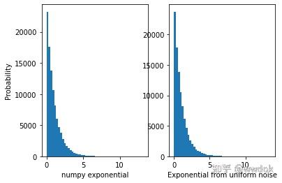

可以看到两个分布十分近似,所以pytorch源代码里使用指数分布采样是没问题的。
3. 注意实现源码中有个hard模式,大多数时候它的默认值是True。
    if hard:

# Straight through.

index = y_soft.max(dim, keepdim=True)[1]

y_hard = torch.zeros_like(logits, memory_format=torch.legacy_contiguous_format).scatter_(dim, index, 1.0)

ret = y_hard - y_soft.detach() + y_soft它里面的ret = y_hard - y_soft.detach() + y_soft是有巧思的,前向传播时, 其中的- y_soft.detach()+y_soft=0,所以ret=y_hard,反向传播时,y_hard是由max和scatter得到的,没有梯度,而- y_soft又detach()了,所以ret=y_soft,所以前向传播和反向传播时是不一样的,而y_hard其实就是one hot的形式,展开说就是index = y_soft.max(dim, keepdim=True)[1] 的作用就是argmax,y_hard = torch.zeros_like(logits, memory_format=torch.legacy_contiguous_format).scatter_(dim, index, 1.0)的作用就是把argmax的结果转成one hot
本文部分内容参考或摘抄自:
《 通俗易懂地理解Gumbel Softmax》
《 gumber分布的维基百科》
《 Gumbel-Softmax 完全解析》
《 Gumbel-Softmax Trick和Gumbel分布 》
《 The Gumbel-Softmax Distribution》
《 Gumbel softmax trick (快速理解附代码)》
《 漫谈重参数:从正态分布到Gumbel Softmax》


 2749
2749


 被折叠的 条评论
为什么被折叠?
被折叠的 条评论
为什么被折叠?
 到【灌水乐园】发言


