R语言绘图ggplot-基本参数

ggplot 框架

#可以省略data =, mapping =, x =, y =
#aes()设定中将变量映射到x、y轴， 颜色、符号、线型等图形元素类型， 也可以作为图形设置将某些图形元素设置为固定值
#fill参数用于指定填充颜色的映射，这意味着你想根据数据集中某个变量的不同取值来区分不同的颜色。
p <- ggplot(data=<输入数据框>, mapping=aes(x=<变量名>,y=<变量名>,color=<变量名>, fill=,size = , alpha = , shape=,<.group=group>/<fill=factor=value.>)) +
#在geom函数中映射变量
#可以在geom_xxx()函数中用mapping = aes(<...>)单独指定变量映射
#注意和ggplot里设置的区别，以及颜色
 geom_<图形类型()geom_point/polygon/>(fill="white", colour = "blue") +
 #坐标刻度值转换函数eg:scale_x_log10(labels=scales::dollar/math/number)
  scale_<映射>_<类型>(<...>) +
  # “类型”包括continuous、discrete、log10
  # scale_y_continuous指定了两个维度的坐标范围
 scale_y_continuous(
    breaks = c(5, 15, 25),
    labels = c("百万分之五", "百万分之十五", "百万分二十五")  )
  coord_<类型>(<...>) +
  labs(
    x = "",
    y = "",
    title = "",
    subtitle = "",
    caption = ""  )+
  geom_smooth(method="lm"/"gam"/"loess")+
  geom_path()#按照输入数据集的次序将坐标点连接在一起
  coord_fixed()#指定两个轴的单位为1:1长度的坐标系， 其中参数xlim和ylim可以指定坐标范围,用expand = FALSE要求坐标轴范围严格等于数据范围或xlim和ylim的规定
   scale_color_brewer(palette = "Set1")
  geom_text(color = "white")

映射

#ggplot()
library(ggplot2)
##准备数据
data(diamonds)	
set.seed(100)
dsmall <-diamonds[sample(nrow(diamonds),100),c(1,2,3,4,7)]
head(dsmall)
p <- ggplot(data = dsmall, 
            mapping = aes(x = carat, y = price))
p0<-p
##几何对象####

p1<-p + geom_point()
p2<-p + geom_point(aes(colour=cut))
p3<-p + geom_point(aes(colour = "blue"))
p4<-p + geom_point(    colour = "blue")
p5<-p + geom_point(aes(colour=cut,shape=clarity))
p6<-p + geom_point(aes(colour=cut,shape=cut))
#~~~~~~~~~~~~~~~
p7 <- 
  p + 
  geom_point(aes(colour=cut), 
             size=5,
             alpha=0.7)
p7

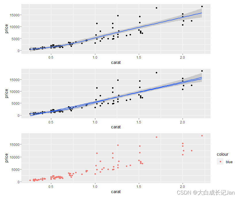
统计变换

p1<-p1 + stat_smooth()
p2<-p1 + stat_smooth(method="lm", 
                 se = FALSE)
P3<-p1 + stat_smooth(method="loess", 
                 se = FALSE,
                 color="red")

p1/p2/p3

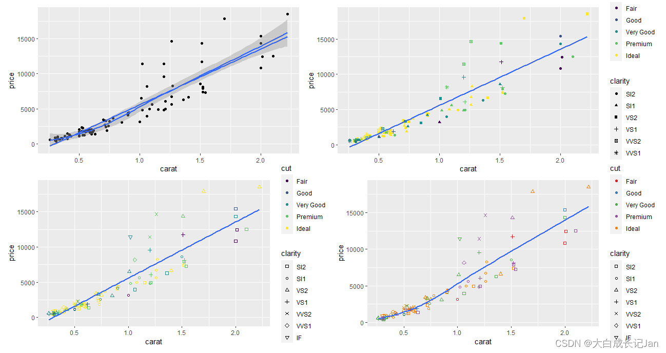
标度

#更改颜色

p1 <-  p1 +
     stat_smooth(method="lm", se = FALSE)
p1 + scale_colour_brewer(palette = "Set1")
#更改形状
p2 <- p + geom_point(aes(colour=cut, shape=clarity)) + 
      stat_smooth(method="lm", se = FALSE)
p3<-p2 + scale_shape_manual(values =0:7)
p4<-p + 
    geom_point(aes(colour=cut, shape=clarity)) + #两个图例
    stat_smooth(method="loess", se = FALSE) + #拟合方式
    scale_colour_brewer(palette = "Set1") + #修改颜色
    scale_shape_manual(values =0:7) #形状修改
(p1+p2)/(p3+p4)

坐标轴变换

#坐标轴转置
p3 <-       
      p1 + 
      scale_colour_brewer(palette = "Set1")
p3
p3 + coord_flip()

调整配色

#install.packages("ggsci")
library(ggsci)
vignette("ggsci")
p4 <- 
  p7+
     theme_classic()
p4

p4 + scale_color_npg()
p4 + scale_color_aaas()
p4 + scale_color_nejm()
p4 + scale_color_lancet()
p4 + scale_color_ucscgb()
p4 + scale_color_d3()
p4 + scale_color_d3(palette = "category20")
p4 + scale_color_startrek()
p4 + scale_color_tron()
p4 + scale_color_simpsons()
p4 + scale_color_locuszoom()
p4 + scale_color_uchicago()
p4 + scale_color_rickandmorty()

调整主题

library(ggthemes)
p4
p4 + theme_solarized() 
p4 + theme_solarized_2(light = FALSE) 
p4 + theme_stata() 
p4 + theme_excel() 
p4 + theme_excel_new() 
p4 + theme_igray()
p4 + theme_fivethirtyeight()
p4 + theme_minimal()
p4 + theme_wsj()
p4 + theme_base()
p4 + theme_pander()
p4 + theme_hc()

p3 + theme_bw()
p3 + theme_grey()
p3 + theme_linedraw()
p3 + theme_light()
p3 + theme_dark()
p3 + theme_minimal()
p3 + theme_classic()
p3 + theme_void()

注释标题

ggplot标题注释

整体参数

ggplot

library(datasets)
data(iris)
summary(iris)
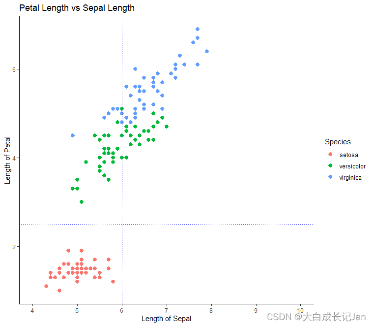
library(ggplot2)
myplot<-ggplot(iris, aes(x=Sepal.Length, y=Petal.Length,color=Species))+
  geom_point(size=2.5)+#手动设置点的大小
  scale_x_continuous(limits=c(4,10),breaks =seq(4,10,1))+#刻度设置
    #Breaks =seq(4,10,1)* → 以 1 的间隔设置从 4 到 10 的刻度
  labs(x = "Length of Sepal",y="Length of Petal" )+#分别设置x轴和y轴
   ggtitle("Petal Length vs Sepal Length")+#标题
   theme_classic()+#设置新主题
   geom_vline(xintercept = 6.0,linetype="dotted",color='blue')+ #添加参考线x=6
   geom_hline(yintercept = 2.5,linetype="dotted",color='blue')

参考R语言教程
数据科学中的R语言
ggplot入门学习
ggplot栅格学习
绘图学习