Stata 回归结果输出之 esttab 详解（更新版）

Policy 是门科学

于 2024-08-02 17:39:46 发布

阅读量675

点赞数 4

分类专栏： Stata 数据处理文章标签：回归数据挖掘

原文链接：https://cloud.tencent.com/developer/article/1820267

版权

Stata 同时被 2 个专栏收录

1 篇文章 0 订阅

订阅专栏

数据处理

1 篇文章 0 订阅

订阅专栏

本文首发于腾讯云：Stata 回归结果输出之 esttab 详解（更新版）

1. 命令简介

esttab 命令是由瑞士波恩大学社会学研究所（University of Bern, Institute of Sociology）的 Ben Jann 教授编写的 Stata 用户外部命令，主要用于生成满足用户需求的回归表格（esttab — Display formatted regression table），这类命令已经成为量化实证分析中的基础性技能，兼具效率、规范与美观。本文是对该命令的详细介绍。
需要说明的是，能够定制化输出统计分析表格的还有其他命令，例如：outreg2、logout 等外部命令，它们的应用逻辑都是一致的，具体选择哪个可根据使用者自己的偏好而定。

2. 命令安装

ssc install estout, replace //estout 是一个通用程序，是 esttab 命令实现其功能的引擎。

3. 使用 esttab 整理回归结果

3.1 基本语法及使用

esttab [ namelist ] [ using filename ] [, options estout_options ]

该命令的使用逻辑如下：

首先，运行单个回归命令并将该模型的估计结果进行存储；
其次，重复上述动作直到所有回归模型均被执行以及所有估计结果均被保存；
最后，使用esttab命令将存储好的估计值或统计量编辑在一个回归表格中；

通过下面的示例进一步掌握：

/* 保存模型结果之方法 I：使用 eststo 命令存储回归模型。
                       通过在回归模型前加上 eststo 前缀，
                       esttab 命令能够自动找到储存的信息，并自动生成对应每个回归模型的变量。*/
   sysuse auto, clear

   eststo: regress price weight mpg         //_est_est1 
   eststo: regress price weight mpg foreign //_est_est2

   esttab //为节省篇幅，提高阅读效率，除非必要，结果不再一一展示，下文不再说明

   eststo clear //删除保存的模型结果，_est_est1 和 _est_est2 从变量窗口中被消失
 
/* 保存模型结果之方法 II：使用 Stata 官方自带的命令进行结果存储，
                        即 estimates store（或缩写形式：est store） */
   sysuse auto, clear

   regress price weight mpg
   estimates store model1

   regress price weight mpg foreign
   estimates store model2

   esttab model1 model2 
   
   //注：此时若使用 eststo clear，保存的结果无法删除

3.2 标准误、P值及概要统计量

esttab的输出结果默认展示带有 t 统计量的的点估计，并在表格注脚处进行标记，一并默认输出的还有样本量。实证研究中，我们往往需要输出估计量的标准误以及其他特定的统计量，这时需要在esttab后进行更为细致的设定。例如，我们需要报告标准误（se）而非 t 统计量，并且需要汇报调整后的判决系数（adj. R-sq）。通过下面的例子，我们可以进一步了解 esttab 命令输出回归结果的设定思路。

sysuse auto, clear
eststo: regress price weight mpg
eststo: regress price weight mpg foreign
esttab, se ar2 /* 跑完回归模型，可以通过 ereturn list 获得该模型的
                  scalars、macros、matrices以及functions */
/*
--------------------------------------------
                      (1)             (2)   
                    price           price   
--------------------------------------------
weight              1.747**         3.465***
                  (0.641)         (0.631)   

mpg                -49.51           21.85   
                  (86.16)         (74.22)   

foreign                            3673.1***
                                  (684.0)   

_cons              1946.1         -5853.7   
                 (3597.0)        (3377.0)   
--------------------------------------------
N                      74              74   
adj. R-sq           0.273           0.478   
--------------------------------------------
Standard errors in parentheses
* p<0.05, ** p<0.01, *** p<0.001 */

esttab, se ar2 nopar nostar //不适用括号以及显著性符号，主要可用于导出至 excel 进行计算
/*
--------------------------------------
                      (1)          (2)
                    price        price
--------------------------------------
weight              1.747        3.465
                    0.641        0.631

mpg                -49.51        21.85
                    86.16        74.22

foreign                         3673.1
                                 684.0

_cons              1946.1      -5853.7
                   3597.0       3377.0
--------------------------------------
N                      74           74
adj. R-sq           0.273        0.478
--------------------------------------
Standard errors in second row */


*上面的命令等价于
 esttab, se scalars(r2_a) //r2_a 是存储在模型估计结果的 scalars中的一个标量参数
 esttab, se stats(r2_a)   //stats() 选项的用法见本文“4.5”部分

/*也可以输出 p 值，置信区间（ci）或是任何存储在估计结果中的参数统计量，
  它们保存在 scalars 中。例如，我们需要输出p值、F统计量以及模型自由度。*/
 esttab, p //以 p 值替换 se
 esttab, p scalars(F df_m df_r)
 eststo clear /*注意，如果把该命令误写为 est sto clear,
                      它表示将上一个回归模型命名为“clear”并储存起来，
                      使用时要理解原理，不断试错才能避免出错. */

3.3 标准化系数

为什么要进行标准化？

同一回归模型中，即便两个自变量的单位一致（例如教育年限和工作经历都以年为计数单位），其回归系数也无法直接进行比较。事实上，研究中涉及的自变量往往具有不同的测度单位，回归系数也会受到影响。

多元回归模型经常涉及各自变量对因变量的相对作用大小进行比较，进而从多个因素中找出首要和次要因素，这时便可以采用标准化的回归系数（standardized coefficients）。所谓标准化回归系数，是将自变量转为一个无量纲的变量，使得不同标准化回归系数之间具有可比性。

随机变量的标准化处理方式

标准化回归系数是通过标准化回归模型估计得到的，需要将模型中所有的自变量和因变量都进行标准化。

将随机变量 X 进行标准化的表达式如下：

$z=\frac{X-E(X)}{\sigma(X)}$

其中， $E (X)$ 和 $\sigma(X)$ 分别表示期望和标准差。z 也叫标准化随机变量或标准分，是一个无量纲的纯数。变量的标准化形式表示：以标准差为单位，测量观测值与均值之间的距离。经过标准化处理后的新变量（z），其均值为0，方差为1。此外，我们还应该知道，标准化处理其实也是一个对中（centering）和测度转换（rescaling）的过程，经过标准化转换，不同变量的位置和尺度得以一致。

估计标准化模型

应用中，我们可以直接将标准化后的变量进行回归，但理论上还是要尽量知其所以然，以便更好理解对标准化模型的估计，很多细节上的问题也自然迎刃而解。假设标准化处理之前的原始回归模型设定如下：

$y_i=\beta_0+\beta_1x_{i1}+\beta_2x_{i2}+…+\beta_px_{ip}+\epsilon_i ~~~~~~~~~~~(1)$

对模型两侧的变量进行标准化转换，即：

$y_{i}^*=\frac{y_{i}-\bar{y}}{S_{y}}$

$x_{ik}^*=\frac{x_{ik}-\bar{x_k}}{S_{xk}}$

对（1）式进行对中处理并除以因变量的标准差 $S_y$ ，模型（1）可做如下变换：

$\frac{y_{i}-\bar{y}}{S_{y}} =\frac{\beta_1}{S_y}(x_{i1}-\bar{x_1})+\frac{\beta_2}{S_y}(x_{i2}-\bar{x_2})+...+\frac{\beta_p}{S_y}(x_{ip}-\bar{x_p})+\frac{\epsilon_i-\bar{\epsilon}}{S_y}$

$~~~~~~~~~=\beta_1\frac{S_{x1}}{S_y}(\frac{x_{i1}-\bar{x_1}}{S_{x1}})+\beta_2\frac{S_{x2}}{S_y}(\frac{x_{i2}-\bar{x_2}}{S_{x2}})+...+\beta_p\frac{S_{xp}}{S_y}(\frac{x_{ip}-\bar{x_p}}{S_{xp}})+\frac{\epsilon_i-\bar{\epsilon}}{S_y}$

$y_i^*= \beta_1^*x_{i1}^*+\beta_2^*x_{i2}^*+...+\beta_p^*x_{ip}^*+\epsilon_i^* ~~~~~~~~~~~~~~~~~~~~(2)$

此时，通过比较模型（1）和模型（2），可以得到标准化与非标准化回归系数之间的关系如下：

$\beta_k^*=\beta_k\times \frac{S{xk}}{S_y}$

显然，利用（3）式，我们也可以通过计算样本中变量 $y$ 与 $x_k$ 的标准差，在获得非标准化系数后求得标准化系数。

两种回归系数的比较

标准化回归系数处于 -1, 1 的取值区间内，并且可以进行标准化尺度下的变量间系数比较。

相比而言，非标准化回归系数虽然不可比，但它将数据本身的信息提供给我们，估计系数具有明确的现实意义。

由此可见，并非进行标准化处理就显得“高大上”，标准化处理与否需要根据所研究的具体问题进行选择。

但是，不论选择哪一种，尤其要关注对两种回归系数的解释。同是边际效应，标准化回归系数表示自变量每增加1个标准差，因变量平均增加 $\beta_k^*$ 个标准差。

使用 esttab 汇报标准化回归系数

sysuse auto, clear
eststo: regress price weight mpg
eststo: regress price weight mpg foreign
esttab
/*汇报常规的非标准化边际效应估计结果
--------------------------------------------
                      (1)             (2)   
                    price           price   
--------------------------------------------
weight              1.747**         3.465***
                   (2.72)          (5.49)   

mpg                -49.51           21.85   
                  (-0.57)          (0.29)   

foreign                            3673.1***
                                   (5.37)   

_cons              1946.1         -5853.7   
                   (0.54)         (-1.73)   
--------------------------------------------
N                      74              74   
--------------------------------------------
t statistics in parentheses
* p<0.05, ** p<0.01, *** p<0.001 */

esttab, beta //也可以汇报标准误，esttab,beta se
/*汇报标准化系数估计结果
--------------------------------------------
                      (1)             (2)   
                    price           price   
--------------------------------------------
weight              0.460**         0.913***
                   (2.72)          (5.49)   

mpg                -0.097           0.043   
                  (-0.57)          (0.29)   

foreign                             0.573***
                                   (5.37)   
--------------------------------------------
N                      74              74   
--------------------------------------------
Standardized beta coefficients; t statistics in parentheses
* p<0.05, ** p<0.01, *** p<0.001*/

esttab, beta not //只汇报标准化系数

3.4 将标准误或 t 统计量在回归系数的右侧汇报

sysuse auto, clear
eststo: regress price weight mpg
eststo: regress price weight mpg foreign
esttab, wide
/*
--------------------------------------------------------------------------------------------------------------------------------
                      (1)                          (2)                          (3)                          (4)                
                    price                        price                        price                        price                
--------------------------------------------------------------------------------------------------------------------------------
weight              1.747**        (2.72)        3.465***       (5.49)        1.747**        (2.72)        3.465***       (5.49)
mpg                -49.51         (-0.57)        21.85          (0.29)       -49.51         (-0.57)        21.85          (0.29)
foreign                                         3673.1***       (5.37)                                    3673.1***       (5.37)
_cons              1946.1          (0.54)      -5853.7         (-1.73)       1946.1          (0.54)      -5853.7         (-1.73)
--------------------------------------------------------------------------------------------------------------------------------
N                      74                           74                           74                           74                
--------------------------------------------------------------------------------------------------------------------------------
t statistics in parentheses
* p<0.05, ** p<0.01, *** p<0.001  */

esttab, se wide //wide 和 se 的顺序可以互换
/*
--------------------------------------------------------------------------------------------------------------------------------
                      (1)                          (2)                          (3)                          (4)                
                    price                        price                        price                        price                
--------------------------------------------------------------------------------------------------------------------------------
weight              1.747**       (0.641)        3.465***      (0.631)        1.747**       (0.641)        3.465***      (0.631)
mpg                -49.51         (86.16)        21.85         (74.22)       -49.51         (86.16)        21.85         (74.22)
foreign                                         3673.1***      (684.0)                                    3673.1***      (684.0)
_cons              1946.1        (3597.0)      -5853.7        (3377.0)       1946.1        (3597.0)      -5853.7        (3377.0)
--------------------------------------------------------------------------------------------------------------------------------
N                      74                           74                           74                           74                
--------------------------------------------------------------------------------------------------------------------------------
Standard errors in parentheses
* p<0.05, ** p<0.01, *** p<0.001 */

3.5 数值的呈现格式

esttab 汇报的回归结果是一个个数值，掌握数值的格式设定规则很有必要。该领命默认格式为a3，上述示例采取的就是默认的数值格式输出，是一种根据每一个统计量自身的数值大小进行的适应性呈现，因此统计量之间便没有统一的格式。可通过设定某一类统计量的数值格式实现更为个性化的输出，具体的实现方式为在要呈现的统计量后加适当的括号()进行格式设定。

sysuse auto, clear
eststo: regress price weight mpg
eststo: regress price weight mpg foreign
esttab, b(a6) p(4) r2(4) nostar wide /*a6表示一种更为精确的格式，
                                       更一般的为a#，#表示有效数字的最小个数，
                                       例子中都是7位有效数字；
                                       4和2分别表示p值和可决系数显示小数点后的位数；
                                       nostar 表示不显示显著性。 */
/*
----------------------------------------------------------------
                      (1)                       (2)             
                    price                     price             
----------------------------------------------------------------
weight           1.746559     (0.0081)     3.464706     (0.0000)
mpg             -49.51222     (0.5673)     21.85360     (0.7693)
foreign                                    3673.060     (0.0000)
_cons            1946.069     (0.5902)    -5853.696     (0.0874)
----------------------------------------------------------------
N                      74                        74             
R-sq               0.2934                    0.4996             
----------------------------------------------------------------
p-values in parentheses
*/

* Stata 官方命令也有专门的格式设定规则，具体可以参见手册：[D] format Set variables’ output format

3.6 标签、标题与注释

esttab 命令可以帮助我们在输出的结果中使用变量标签表示变量，这非常实用，也有利于我们在数据处理阶段重识对标签的管理，规范的标签设置可以帮助我们更清楚且更有效地呈现回归结果。

sysuse auto, clear
eststo: regress price weight mpg
eststo: regress price weight mpg foreign
esttab, se label title(Tabel. Regression results) ///
        nonumbers mtitles("Model A" "Model B")    /// 
        addnote("Source: auto.dta from Stata's System")
/*
Tabel. Regression results
----------------------------------------------------
                          Model A         Model B   
----------------------------------------------------
Weight (lbs.)               1.747**         3.465***
                          (0.641)         (0.631)   

Mileage (mpg)              -49.51           21.85   
                          (86.16)         (74.22)   

Car type                                   3673.1***
                                          (684.0)   

Constant                   1946.1         -5853.7   
                         (3597.0)        (3377.0)   
----------------------------------------------------
Observations                   74              74   
----------------------------------------------------
Standard errors in parentheses
Source: auto.dta from Stata's System
* p<0.05, ** p<0.01, *** p<0.001                  */

* 注： [no]numbers：do not/do print model numbers in table header

此外，label 选项还支持因子变量（factor variables）和交互项（interaction terms ）。

sysuse auto, clear
eststo: regress price mpg i.foreign
eststo: regress price c.mpg##i.foreign
esttab 
/*
--------------------------------------------
                      (1)             (2)   
                    price           price   
--------------------------------------------
mpg                -294.2***       -329.3***
                  (-5.28)         (-4.39)   

0.foreign               0               0   
                      (.)             (.)   

1.foreign          1767.3*         -13.59   
                   (2.52)         (-0.01)   

0.foreign#~g                            0   
                                      (.)   

1.foreign#~g                        78.89   
                                   (0.70)   

_cons             11905.4***      12600.5***
                  (10.28)          (8.25)   
--------------------------------------------
N                      74              74   
--------------------------------------------
t statistics in parentheses
* p<0.05, ** p<0.01, *** p<0.001          */

esttab, varwidth(20) //修改允许呈现的变量宽度，可根据呈现效果调整
/*
----------------------------------------------------
                              (1)             (2)   
                            price           price   
----------------------------------------------------
mpg                        -294.2***       -329.3***
                          (-5.28)         (-4.39)   

0.foreign                       0               0   
                              (.)             (.)   

1.foreign                  1767.3*         -13.59   
                           (2.52)         (-0.01)   

0.foreign#c.mpg                                 0   
                                              (.)   

1.foreign#c.mpg                             78.89   
                                           (0.70)   

_cons                     11905.4***      12600.5***
                          (10.28)          (8.25)   
----------------------------------------------------
N                              74              74   
----------------------------------------------------
t statistics in parentheses
* p<0.05, ** p<0.01, *** p<0.001                  */

esttab, varwidth(25) label
/*
---------------------------------------------------------
                                   (1)             (2)   
                                 Price           Price   
---------------------------------------------------------
Mileage (mpg)                   -294.2***       -329.3***
                               (-5.28)         (-4.39)   

Domestic                             0               0   
                                   (.)             (.)   

Foreign                         1767.3*         -13.59   
                                (2.52)         (-0.01)   

Domestic # Mileage (mpg)                             0   
                                                   (.)   

Foreign # Mileage (mpg)                          78.89   
                                                (0.70)   

Constant                       11905.4***      12600.5***
                               (10.28)          (8.25)   
---------------------------------------------------------
Observations                        74              74   
---------------------------------------------------------
t statistics in parentheses
* p<0.05, ** p<0.01, *** p<0.001                       */

esttab, varwidth(25) label nobaselevels interaction(" X ")
/*
---------------------------------------------------------
                                   (1)             (2)   
                                 Price           Price   
---------------------------------------------------------
Mileage (mpg)                   -294.2***       -329.3***
                               (-5.28)         (-4.39)   

Foreign                         1767.3*         -13.59   
                                (2.52)         (-0.01)   

Foreign X Mileage (mpg)                          78.89   
                                                (0.70)   

Constant                       11905.4***      12600.5***
                               (10.28)          (8.25)   
---------------------------------------------------------
Observations                        74              74   
---------------------------------------------------------
t statistics in parentheses
* p<0.05, ** p<0.01, *** p<0.001                       */

* 还可以直接输出纯文本表格的结果
  esttab, plain /*需要注意的是，纯文本输出没有显著性标记，
                  但这种方式也有其优点，例如，结果输出到excel后可直接开展进一步计算。 */
  *(output omitted)

3.7 压缩行距的表格

sysuse auto, clear
eststo: regress price weight mpg
eststo: regress price weight mpg foreign
eststo: regress price weight mpg foreign displacement
esttab
/*
------------------------------------------------------------
                      (1)             (2)             (3)   
                    price           price           price   
------------------------------------------------------------
weight              1.747**         3.465***        2.458** 
                   (2.72)          (5.49)          (2.82)   

mpg                -49.51           21.85           19.08   
                  (-0.57)          (0.29)          (0.26)   

foreign                            3673.1***       3930.2***
                                   (5.37)          (5.67)   

displacement                                        10.22   
                                                   (1.65)   

_cons              1946.1         -5853.7         -4846.8   
                   (0.54)         (-1.73)         (-1.43)   
------------------------------------------------------------
N                      74              74              74   
------------------------------------------------------------
t statistics in parentheses
* p<0.05, ** p<0.01, *** p<0.001                          */

esttab, compress //compress reduces the amount of horizontal spacing
/*
-------------------------------------------------
                 (1)          (2)          (3)   
               price        price        price   
-------------------------------------------------
weight         1.747**      3.465***     2.458** 
              (2.72)       (5.49)       (2.82)   

mpg           -49.51        21.85        19.08   
             (-0.57)       (0.29)       (0.26)   

foreign                    3673.1***    3930.2***
                           (5.37)       (5.67)   

displace~t                               10.22   
                                        (1.65)   

_cons         1946.1      -5853.7      -4846.8   
              (0.54)      (-1.73)      (-1.43)   
-------------------------------------------------
N                 74           74           74   
-------------------------------------------------
t statistics in parentheses
* p<0.05, ** p<0.01, *** p<0.001               */

3.8 系数显著性的星标设定

正如上面的示例所示，显著性标记默认的输出符号和阈值为：

* for p<.05
** for p<.01
*** for p<.001

因此，根据统计分析的规范，需要对显著性的标记进行重新设定，调整为 *0.10、**0.05、***0.01。我们也可以手动设定复合需要的显著性水平，亦可通过nostar选项不显示显著性标记。

sysuse auto, clear
eststo: regress price weight mpg
eststo: regress price weight mpg foreign
esttab, star( *0.10 ** 0.05 *** 0.01)  //显著性常规设定
/*
--------------------------------------------
                      (1)             (2)   
                    price           price   
--------------------------------------------
weight              1.747***        3.465***
                  (0.641)         (0.631)   

mpg                -49.51           21.85   
                  (86.16)         (74.22)   

foreign                            3673.1***
                                  (684.0)   

_cons              1946.1         -5853.7*  
                 (3597.0)        (3377.0)   
--------------------------------------------
N                      74              74   
--------------------------------------------
Standard errors in parentheses
* p<0.10, ** p<0.05, *** p<0.01 */


esttab, star( & 0.10 * 0.05)   //用什么符号完全可以自己随心所欲地设定，+、-、&、%.....均可
/*

----------------------------------------
                      (1)           (2) 
                    price         price 
----------------------------------------
weight              1.747*        3.465*
                  (0.641)       (0.631) 

mpg                -49.51         21.85 
                  (86.16)       (74.22) 

foreign                          3673.1*
                                (684.0) 

_cons              1946.1       -5853.7&
                 (3597.0)      (3377.0) 
----------------------------------------
N                      74            74 
----------------------------------------
Standard errors in parentheses
& p<0.10, * p<0.05     */

4. 使用 esttab 输出回归表格

使用 esttab 命令的最终目的在于将回归结果呈现于工作文档之中。

4.1 输出至 Excel

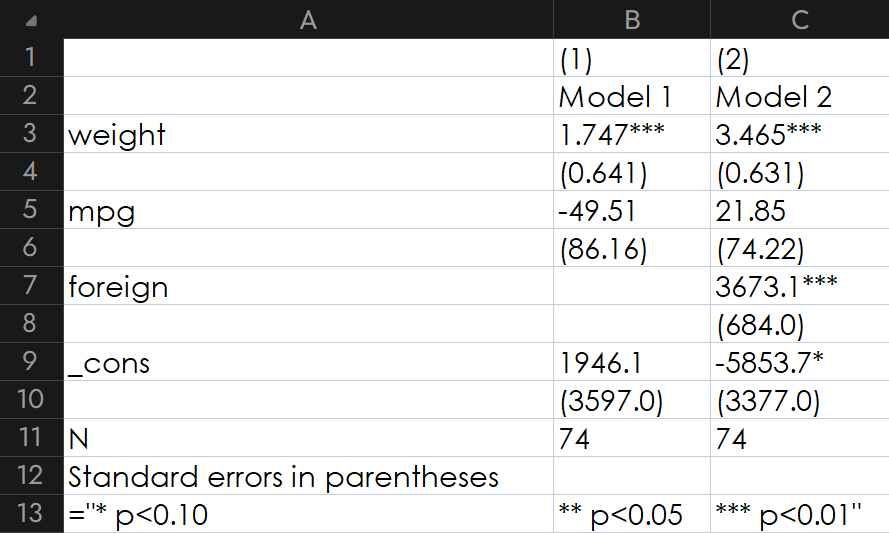
通过设定一个后缀为.csv文件格式的文件名，可以将结果输出为 excel 可读的的文档。

sysuse auto, clear
eststo: regress price weight mpg
eststo: regress price weight mpg foreign
esttab using excel_demmo.csv, mtitles("Model 1" "Model 2")        ///
                              se star( * 0.10 ** 0.05 *** 0.01)   ///
                              nogap replace //可根据上文列出的相关命令进行更多定制化的设定

图 1. 输出规范的回归结果至 Excel 文档

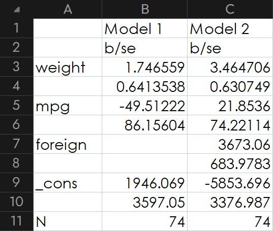
如果要对回归结果进行其他处理（例如，计算变量之间的边际替代率或绘图等），可以输出为纯文本格式：

esttab using excel_demmo.csv, mtitles("Model 1" "Model 2")        ///
                              se nostar                           ///
                              plain nogap replace //可根据上文列出的相关命令进行更多定制化的设定

图 2. 输出纯文本回归结果至 Excel 文档（便于进一步计算）

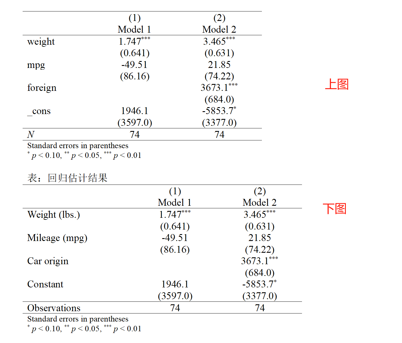
4.2 输出至 Word

通过设定一个后缀为.rft文件格式的文件名，可以将结果输出为 word 可读的的文档。

进一步，可以使用 append 选项将新的输出内容添加到已经输出的文档之中。

另一个很实用的选项是 onecell，能够把点估计的t值和标准误直接置于位于同一个表格的格子内。

.rft 是Rich Text Format（RFT）的缩写，意即丰富的文本格式。在rtf文档中可以嵌入图像等文件，RTF是word为了与其他字处理软件兼容而能够保存的文档格式，类似 doc 格式（Word文档）的文件，有很好的兼容性。

sysuse auto, clear
eststo: regress price weight mpg
eststo: regress price weight mpg foreign
//上图
esttab using excel_demmo.rtf, mtitles("Model 1" "Model 2")        ///
                              se star( * 0.10 ** 0.05 *** 0.01)   ///
                              nogap replace 
//下图    
esttab using excel_demmo.rtf, title("表：回归估计结果") mtitles("Model 1" "Model 2")   ///
                              se star( * 0.10 ** 0.05 *** 0.01)   ///
                              nogap label onecell replace         ///
                              append

图 3. 使用 onecell 下添加 nogap 选项与否的输出结果比较

4.3 非标准内容的输出

esttab通过预先定义好的选项输出特定的参数统计量，但有时我们需要输出其他统计量。可以通过main()和aux()选项分别实现对“点估计”和“t值/标准误”的替换。

下面以回归后将默认的 t 统计量替换为方差膨胀因子（Variance Inflation Factors, VIF）为例进行说明。

sysuse auto, clear
eststo: regress price weight mpg foreign
*estat vif   //显示计算结果但未存储至估计结果矩阵
estadd vif   //显示相同计算结果并且存储至估计结果矩阵
ereturn list //查看 “ matrices: ” 下的 “ e(vif) :  1 x 4 ”

esttab, b(3) aux(vif 3) star(* 0.10 ** 0.05 *** 0.01)
        wide nopar   //the aux() option to replace the t-statistics
              //the statistics stored in e(name)
              //aux() 中的第二个元素用于设定小数点后的位数
              //[no]parentheses: do not/do print parentheses around t-statistics；默认圆括号 ()。
/*
-----------------------------------------
                      (1)                
                    price                
-----------------------------------------
weight              3.465***        3.864
mpg                21.854           2.965
foreign          3673.060***        1.593
_cons           -5853.696*               
-----------------------------------------
N                      74                
-----------------------------------------
vif in second column
* p<0.10, ** p<0.05, *** p<0.01 */      

esttab, b(3) aux(vif 3) star(* 0.10 ** 0.05 *** 0.01)  ///
        wide bracket  //将圆括号 () 替换为方括号 []                        
/*
-----------------------------------------
                      (1)                
                    price                
-----------------------------------------
weight              3.465***      [3.864]
mpg                21.854         [2.965]
foreign          3673.060***      [1.593]
_cons           -5853.696*               
-----------------------------------------
N                      74                
-----------------------------------------
vif in brackets
* p<0.10, ** p<0.05, *** p<0.01 */

更一般地，我们可能希望展示超过两个以上的参数统计量。

例如，像之前一样汇报变量的点估计量和 t 值，同时汇报每个变量的方差膨胀因子（vif），这时需要借助于estout语法规则（如开篇所述，esttab 是estout的一个子命令），具体使用cells()选项进行设定。

值得一提的是，estout中所有的选项都可以在esttab中使用，且相对于后者自身的选项而言优先被执行。例如，若设定了cells()，则main()，se()，t()，p()，aux()，star，wide，onecell等上面使用过的选项都将失效。

关于如何使用cell()，下面做简要介绍：

sysuse auto, clear
eststo: regress price weight mpg foreign
estadd vif

esttab, b(3) se(2) star( * 0.10 ** 0.05 *** 0.01) nogap
/*
----------------------------
                      (1)   
                    price   
----------------------------
weight              3.465***
                   (0.63)   
mpg                21.854   
                  (74.22)   
foreign          3673.060***
                 (683.98)   
_cons           -5853.696*  
                (3376.99)   
----------------------------
N                      74   
----------------------------
Standard errors in parentheses
* p<0.10, ** p<0.05, *** p<0.01 */

esttab, cells( "b(fmt(3) star)" se(par fmt(2))) /// * fmt:specify the format(s) of a statistic
        star(* 0.10 ** 0.05 *** 0.01)  //与上方命令等价
/*
----------------------------
                      (1)   
                    price   
                     b/se   
----------------------------
weight              3.465***
                   (0.63)   
mpg                21.854   
                  (74.22)   
foreign          3673.060***
                 (683.98)   
_cons           -5853.696*  
                (3376.99)   
----------------------------
N                      74   
---------------------------- */

esttab, b(3) se(2) star( * 0.10 ** 0.05 *** 0.01) nogap wide
/*
-----------------------------------------
                      (1)                
                    price                
-----------------------------------------
weight              3.465***       (0.63)
mpg                21.854         (74.22)
foreign          3673.060***     (683.98)
_cons           -5853.696*      (3376.99)
-----------------------------------------
N                      74                
-----------------------------------------
Standard errors in parentheses
* p<0.10, ** p<0.05, *** p<0.01 */

esttab, cells( "b(fmt(3) star) se(par fmt(2))") /// 
        star(* 0.10 ** 0.05 *** 0.01)  //与上方命令等价           
/*
-----------------------------------------
                      (1)                
                    price                
                        b              se
-----------------------------------------
weight              3.465***       (0.63)
mpg                21.854         (74.22)
foreign          3673.060***     (683.98)
_cons           -5853.696*      (3376.99)
-----------------------------------------
N                      74                
----------------------------------------- */

esttab, cells( "b(fmt(3) star) vif(fmt(3))" se(par fmt(2)))  ///
        star(* 0.10 ** 0.05 *** 0.01)  
/*-----------------------------------------
                      (1)                
                    price                
                     b/se             vif
-----------------------------------------
weight              3.465***        3.864
                   (0.63)                
mpg                21.854           2.965
                  (74.22)                
foreign          3673.060***        1.593
                 (683.98)                
_cons           -5853.696*               
                (3376.99)                
-----------------------------------------
N                      74                
----------------------------------------- */


esttab, cells( "b(fmt(3) star) vif(fmt(3))" se(par fmt(2)) t(par fmt(2)))  ///
        star(* 0.10 ** 0.05 *** 0.01)  
/*
-----------------------------------------
                      (1)                
                    price                
                   b/se/t             vif
-----------------------------------------
weight              3.465***        3.864
                   (0.63)                
                   (5.49)                
mpg                21.854           2.965
                  (74.22)                
                   (0.29)                
foreign          3673.060***        1.593
                 (683.98)                
                   (5.37)                
_cons           -5853.696*               
                (3376.99)                
                  (-1.73)                
-----------------------------------------
N                      74                
----------------------------------------- */

4.4 固定效应的 YES or NO

固定效应或不可观测效应（ Fixed/ Unobserved Effects）是计量经济学中一个常见概念。对任何个体单元而言，能够影响因变量的不可观测特征至少在一定时期内不会随时间而变化。例如，个体的价值观、能力、口味偏好等仅在个体间存在差异但又无法观测的特征。

在应用中，通常使用虚拟变量的方式对固定效应进行控制，研究者或审稿人往往不纠结于这些虚拟变量的系数，因而在回归表格中往往只需要告诉读者是否（YES or NO）对这些重要的效应进行了控制。

使用esttab 命令展示是否控制固定效应十分便捷，可由下面的例子直观呈现：

sysuse nlsw88.dta, clear
eststo: reg wage age ttl_exp hours i.collgrad i.occupation i.industry
esttab, se star(* 0.10 ** 0.05 *** 0.01)   ///
        nobaselevels indicate("职业固定效应 =*.occupation" "行业固定效应 =*.industry" ) 

/*呈现结果如下
------------------------------------------------------------
                      (1)             (2)             (3)   
                     wage            wage            wage   
------------------------------------------------------------
age               -0.0928**       -0.0915**       -0.0743** 
                 (0.0363)        (0.0368)        (0.0358)   

ttl_exp             0.228***        0.236***        0.185***
                 (0.0255)        (0.0259)        (0.0256)   

hours              0.0287**        0.0375***       0.0195*  
                 (0.0112)        (0.0111)        (0.0111)   

1.collgrad          2.637***        3.471***        2.746***
                  (0.318)         (0.281)         (0.315)   

_cons               8.793***        4.690**         8.544***
                  (1.508)         (1.977)         (2.083)   

职业固定效应          Yes              No             Yes   

行业固定效应           No             Yes             Yes   
------------------------------------------------------------
N                    2233            2228            2224   
------------------------------------------------------------
Standard errors in parentheses
* p<0.10, ** p<0.05, *** p<0.01  */

4.5 在回归表格中添加重要统计量

一张符合规范的回归表格除了回归系数、标准误/t值、样本量（N）等信息外，还应包含或可包含一些重要的统计量。在回归表格中添加这些重要的统计量可使得回归表格更具自我说明性，使用stats()选项便可快速实现重要统计量的添加。

事实上，这些能够被添加的统计量是标量（Scalars），所谓标量，就是只有大小没有方向的一些东西。执行回归命令后，模型估计所产生的各类标量统计量会被存储起来，我们在结果窗口中只是看到其中的一部分而已。具体地，这些标量主要包含以下内容：

赤池信息准则 (Akaike’s information criterion, AIC)
贝叶斯信息准则（Bayesian/Schwarz’s information criterion, BIC)
模型秩的数量 (the rank of e(V), i.e. the number of free parameters in model)
模型 P 值 (the p-value of the model)
其他储存起来的模型的标量；执行回归后可通过ereturn list获得。

* 有关 AIC 和 BIC 的定义和异同可参考此文：模型中AIC和BIC以及loglikelihood的关系

在下面的例子中，我们先来看一看执行回归命令后有哪些标量统计量被储存了起来：

sysuse auto, clear
regress price weight mpg foreign
ereturn list
/* scalars:
                  e(N) =  74
               e(df_m) =  3
               e(df_r) =  70
                  e(F) =  23.29224584461625
                 e(r2) =  .4995593889723035
               e(rmse) =  2130.769528589715
                e(mss) =  317252881.2439712
                e(rss) =  317812514.8776504
               e(r2_a) =  .4781119342139736
                 e(ll) =  -670.0990140763248
               e(ll_0) =  -695.7128688987767
               e(rank) =  4

   macros:
            e(cmdline) : "regress price weight mpg foreign"
              e(title) : "Linear regression"
          e(marginsok) : "XB default"
                e(vce) : "ols"
             e(depvar) : "price"
                e(cmd) : "regress"
         e(properties) : "b V"
            e(predict) : "regres_p"
              e(model) : "ols"
          e(estat_cmd) : "regress_estat"

  matrices:
                  e(b) :  1 x 4
                  e(V) :  4 x 4

  functions:
             e(sample)   */

知道了有那些标量统计量，接下来的任务就是在 esttab 命令中使用 stats() 选项将其展示出来。事实上，我们不仅可以展示模型的标量统计量，与模型对应的宏（Macro）信息也可以被列示出来。

sysuse auto, clear
eststo: regress price weight mpg foreign
eststo: regress price weight mpg foreign, robust
eststo: regress price weight mpg foreign, vce(bootstrap)

esttab, se star(* 0.10 ** 0.05 *** 0.01)   ///
        label varlabels(_cons 常数项)      ///
        stats(N r2 r2_a aic bic vce)      
        
/*呈现结果如下

--------------------------------------------------------------------
                              (1)             (2)             (3)   
                            Price           Price           Price   
--------------------------------------------------------------------
Weight (lbs.)               3.465***        3.465***        3.465***
                          (0.631)         (0.778)         (0.781)   
Mileage (mpg)               21.85           21.85           21.85   
                          (74.22)         (80.75)         (84.92)   
Car origin                 3673.1***       3673.1***       3673.1***
                          (684.0)         (664.9)         (729.7)   
常数项                    -5853.7*        -5853.7         -5853.7   
                         (3377.0)        (3873.7)        (3955.1)   
--------------------------------------------------------------------
N                              74              74              74   
r2                          0.500           0.500           0.500   
r2_a                        0.478           0.478           0.478   
aic                        1348.2          1348.2          1348.2   
bic                        1357.4          1357.4          1357.4   
vce                           ols          robust       bootstrap   
--------------------------------------------------------------------
Standard errors in parentheses
* p<0.10, ** p<0.05, *** p<0.01   */

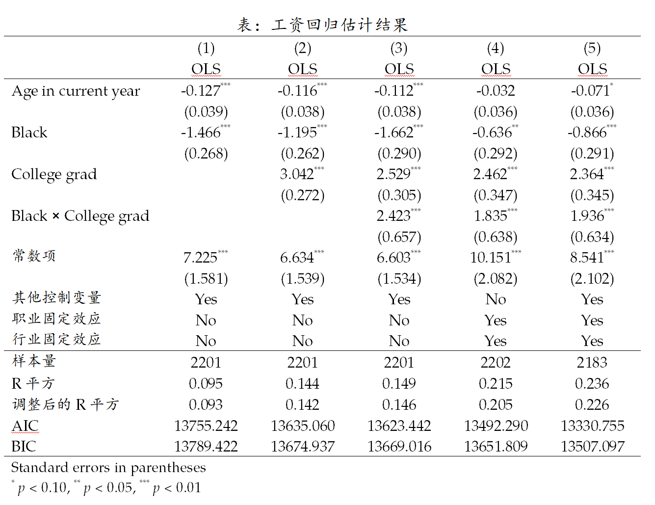
5. 一个整合的回归结果输出模板

基于前文对 esttab 命令各个部件的功能详解，我们以个体工资是否存在种族歧视以及上大学是否能否缓解工资水平在种族间的差异为例，可以形成一个整合的命令模板如下：

clear all 
sysuse nlsw88.dta, clear
drop if race == 3
global cons "hours ttl_exp tenure"
eststo: reg wage age i.race $cons
eststo: reg wage age i.race i.collgrad $cons
eststo: reg wage age i.race i.collgrad i.race#i.collgrad $cons
eststo: reg wage age i.race i.collgrad i.race#i.collgrad i.occupation i.industry
eststo: reg wage age i.race i.collgrad i.race#i.collgrad i.occupation i.industry $cons

esttab using module.rtf, title("表：工资回归估计结果") mtitles("OLS" "OLS" "OLS" "OLS" "OLS")   ///
                         b(3) se(3) star(* 0.10 ** 0.05 *** 0.01)                             ///
                         varwidth(25) label onecell nogap nobaselevels interaction(" X ") varlabels(_cons 常数项)      ///
                         stats(N r2 r2_a aic bic, fmt(0 3 3 3 3) labels("样本量" "R平方" "调整后的R平方" "AIC" "BIC"))  ///
                         indicate("其他控制变量=$cons" "职业固定效应 =*.occupation" "行业固定效应 =*.industry")          ///
                         replace

图 4. 模板示例的估计结果

6. 更多应用示例

6.1 在 logit 回归中输出指数化系数

*Exponentiated Coefficients

sysuse auto, clear
eststo: logit    foreign mpg weight //Coefficient
eststo: logistic foreign mpg weight //Odds ratio
esttab //不论模型如何，只汇报系数
/*
--------------------------------------------
                      (1)             (2)   
                  foreign         foreign   
--------------------------------------------
foreign                                     
mpg                -0.169          -0.169   
                  (-1.83)         (-1.83)   

weight           -0.00391***     -0.00391***
                  (-3.86)         (-3.86)   

_cons               13.71**         13.71** 
                   (3.03)          (3.03)   
--------------------------------------------
N                      74              74   
--------------------------------------------
t statistics in parentheses
* p<0.05, ** p<0.01, *** p<0.001 */

dis exp(-0.1685869) // = .84485784
esttab, eform       //不论模型如何，只汇报指数化系数
/*
--------------------------------------------
                      (1)             (2)   
                  foreign         foreign   
--------------------------------------------
foreign                                     
mpg                 0.845           0.845   
                  (-1.83)         (-1.83)   

weight              0.996***        0.996***
                  (-3.86)         (-3.86)   
--------------------------------------------
N                      74              74   
--------------------------------------------
Exponentiated coefficients; t statistics in parentheses
* p<0.05, ** p<0.01, *** p<0.001 */

esttab, mtitles("logit" "logistic") eform(0 1)  //对应模型是否使用指数化系数
/*
--------------------------------------------
                      (1)             (2)   
                    logit        logistic   
--------------------------------------------
foreign                                     
mpg                -0.169           0.845   
                  (-1.83)         (-1.83)   

weight           -0.00391***        0.996***
                  (-3.86)         (-3.86)   

_cons               13.71**      898396.7** 
                   (3.03)          (3.03)   
--------------------------------------------
N                      74              74   
--------------------------------------------
t statistics in parentheses
* p<0.05, ** p<0.01, *** p<0.001    */

6.2 输出边际效应

sysuse auto, clear
generate reprec = (rep78 > 3) if rep78<.
eststo: logit foreign mpg reprec
eststo: mfx
esttab, se margin mtitles("coefficients" "marginal effects")

/*
--------------------------------------------
                      (1)             (2)   
             coefficients    marginal e~s   
--------------------------------------------
foreign                                     
mpg                 0.140*         0.0240*  
                 (0.0653)        (0.0121)   

reprec (d)          2.650***        0.481***
                  (0.738)         (0.113)   
--------------------------------------------
N                      69              69   
--------------------------------------------
Marginal effects; Standard errors in parentheses
 (d) for discrete change of dummy variable from 0 to 1
* p<0.05, ** p<0.01, *** p<0.001 */

6.3 多方程估计（Heckman \ Sureg \ IV）

//Heckman样本选择模型
webuse womenwk, clear
nmissing wage //wage 657（缺失值数量）
gen employed =(wage !=.)

eststo OLS:     reg wage educ age 
eststo MLE:     heckman wage educ age, select(married children educ age) 
eststo Towstep: heckman wage educ age, select(married children educ age) twostep

eststo Heck1: probit employed married children educ age
        predict y_hat, xb  // xb: calculate linear prediction
        gen pdf = normalden(y_hat) 
        gen cdf = normal(y_hat)
        gen imr = pdf/cdf  //计算逆米尔斯比率
eststo Heck2: reg  wage educ age imr if employed == 1

esttab, mtitles se(2) 
/*
--------------------------------------------------------------------------------------------
                      (1)             (2)             (3)             (4)             (5)   
                      OLS             MLE         Towstep           Heck1           Heck2   
--------------------------------------------------------------------------------------------
main                                                                                        
education           0.897***        0.990***        0.983***       0.0584***        0.983***
                   (0.05)          (0.05)          (0.05)          (0.01)          (0.05)   

age                 0.147***        0.213***        0.212***       0.0347***        0.212***
                   (0.02)          (0.02)          (0.02)          (0.00)          (0.02)   

married                                                             0.431***                
                                                                   (0.07)                   

children                                                            0.447***                
                                                                   (0.03)                   

imr                                                                                 4.002***
                                                                                   (0.58)   

_cons               6.085***        0.486           0.734          -2.467***        0.734   
                   (0.89)          (1.08)          (1.25)          (0.19)          (1.17)   
--------------------------------------------------------------------------------------------
select                                                                                      
married                             0.445***        0.431***                                
                                   (0.07)          (0.07)                                   

children                            0.439***        0.447***                                
                                   (0.03)          (0.03)                                   

education                          0.0557***       0.0584***                                
                                   (0.01)          (0.01)                                   

age                                0.0365***       0.0347***                                
                                   (0.00)          (0.00)                                   

_cons                              -2.491***       -2.467***                                
                                   (0.19)          (0.19)                                   
--------------------------------------------------------------------------------------------
/                                                                                           
athrho                              0.874***                                                
                                   (0.10)                                                   

lnsigma                             1.793***                                                
                                   (0.03)                                                   
--------------------------------------------------------------------------------------------
/mills                                                                                      
lambda                                              4.002***                                
                                                   (0.61)                                   
--------------------------------------------------------------------------------------------
N                    1343            2000            2000            2000            1343   
--------------------------------------------------------------------------------------------
Standard errors in parentheses
* p<0.05, ** p<0.01, *** p<0.001 */


// 似不相关回归
sysuse auto, clear
sureg (price foreign weight length) (mpg displ = foreign weight)
esttab, se wide
esttab, se unstack  //place multiple equations in separate columns
esttab, se unstack scalars(r2 chi2 p) noobs nomtitle 
*结果不再展示


//工具变量的两阶段最小二乘法估计
*使用ivregress2（stata自带的2SLS命令为 ivregress 2sls，无法输出第1阶段回归结果）
eststo clear
use "https://www.stata-press.com/data/r17/hsng", clear
eststo: reg rent hsngval pcturban
eststo: reg hsngval faminc i.region pcturban
eststo: ivregress2 2sls rent pcturban (hsngval = faminc i.region) 

estat endogenous   //Tests of endogeneity(H0: Variables are exogenous)
return list
estadd scalar Durbin = `r(durbin)'  //文本用 local 
ereturn list

esttab, mtitles("OLS" "IV-First" "2SLS") nobaselevels se replace ///
        stats(N r2 r2_a Durbin, fmt(0 3 3 3) labels("样本量" "R2" "调整后的R2" "Durbin"))
/*
------------------------------------------------------------
                      (1)             (2)             (3)   
                      OLS        IV-First            2SLS   
------------------------------------------------------------
hsngval           0.00152***                      0.00224***
               (0.000228)                      (0.000328)   

pcturban            0.525*          182.2          0.0815   
                  (0.249)         (115.0)         (0.299)   

faminc                              2.731***                
                                  (0.682)                   

2.region                          -5095.0                   
                                 (4122.1)                   

3.region                          -1778.1                   
                                 (4072.7)                   

4.region                          13413.8**                 
                                 (4048.1)                   

_cons               125.9***     -18671.9           120.7***
                  (14.19)       (11995.5)         (15.23)   
------------------------------------------------------------
样本量                 50              50              50   
R2                  0.669           0.691           0.599   
调整后的R2          0.655           0.656           0.582   
Durbin                                             12.847   
------------------------------------------------------------
Standard errors in parentheses
* p<0.05, ** p<0.01, *** p<0.001 */


*使用 ivreg2
eststo clear
use "https://www.stata-press.com/data/r17/hsng", clear
eststo OLS: reg rent hsngval pcturban
eststo IV: ivreg2 rent pcturban (hsngval = faminc i.region), first savefirst savefprefix(first_)
esttab first_hsngval IV
/*与上面的结果一致 */

6.4 效应符号

sysuse auto, clear
eststo: regress price mpg foreign
eststo: regress price mpg foreign weight

esttab, cells(_sign)
/*
--------------------------------------
                      (1)          (2)
                    price        price
                    _sign        _sign
--------------------------------------
mpg                     -            +
foreign                 +            +
weight                               +
_cons                   +            -
--------------------------------------
N                      74           74
-------------------------------------- */

esttab, cells(_star) ///
        starlevels(* 0.1 ** 0.05 *** 0.01)
/*
--------------------------------------
                      (1)          (2)
                    price        price
                    _star        _star
--------------------------------------
mpg                   ***             
foreign                **          ***
weight                             ***
_cons                 ***            *
--------------------------------------
N                      74           74
-------------------------------------- */

esttab, cells(_sigsign)  ///
        starlevels("+/-" 0.1 "++/--" 0.05 "+++/---" 0.01)
/*
--------------------------------------
                      (1)          (2)
                    price        price
                 _sigsign     _sigsign
--------------------------------------
mpg                   ---             
foreign                ++          +++
weight                             +++
_cons                 +++            -
--------------------------------------
N                      74           74
-------------------------------------- */

6.5 添加假设预期方向

sysuse auto, clear
reg price mpg foreign weight displacement
esttab, labcol2(+ ? + -, title("方向" Hypothesis))
/*
-----------------------------------------
                 方向              (1)   
              Hypothesis         price   
-----------------------------------------
mpg               +              19.08   
                                (0.26)   

foreign           ?             3930.2***
                                (5.67)   

weight            +              2.458** 
                                (2.82)   

displacement      -              10.22   
                                (1.65)   

_cons                          -4846.8   
                               (-1.43)   
-----------------------------------------
N                                   74   
-----------------------------------------
t statistics in parentheses
* p<0.05, ** p<0.01, *** p<0.001 */

本文首发于腾讯云：Stata 回归结果输出之 esttab 详解（更新版）

过往版本2021-05-04；2023-05-23；2024-07-29

最新版本2024-07-30

更新次数3

Policy 是门科学

关注

4
点赞
踩
4

收藏

觉得还不错? 一键收藏
0
评论
Stata 回归结果输出之 esttab 详解（更新版）

本文首发于腾讯云：Stata 回归结果输出之 esttab 详解（更新版） esttab 命令是由瑞士波恩大学社会学研究所（University of Bern, Institute of Sociology）的 Ben Jann 教授编写的用户外部命令，主要用于生成满足用户需求的回归表格（esttab — Display formatted regression table），这类命令已经成为量化实证分析中的基础性技能，兼具效率、规范与美观。结合实例，本文是对该命令的一份详细介绍。
复制链接

扫一扫