【论文精读】Semi-supervised Medical Image Segmentation through Dual-task Consistency

LANG_C_

已于 2023-05-09 09:09:35 修改

阅读量2.4k

点赞数 5

分类专栏：论文精读

于 2022-07-07 21:32:31 首次发布

本文链接：https://blog.csdn.net/weixin_45648030/article/details/125665476

版权

半监督学习医学图像分割双任务一致性水平集函数深度学习

关键词由CSDN通过智能技术生成

论文精读专栏收录该内容

16 篇文章 12 订阅

订阅专栏

语义分割论文

CVPR 2021 基于双任务一致性的半监督医学图像分割代码：

GitHub - HiLab-git/DTC: Semi-supervised Medical Image Segmentation through Dual-task Consistency

1.Dual-task Consistency

2.Semi-supervised training through Dual-Task-Consistency

3. Algorithm

三、实验部分

1.胰腺CT数据集上双任务一致性方法的消融研究

2.与其他半监督方法的比较

总结

摘要

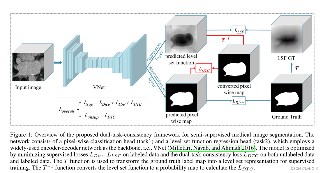
基于深度学习的半监督学习(SSL)算法在医学图像分割方面取得了很有前景的结果，可以通过利用未标记的数据来减轻医生昂贵的注释。然而，文献中现有的SSL算法大多倾向于通过扰动网络或数据来regularize模型训练。观察到多任务/双任务学习关注具有固有预测扰动的不同级别的信息，我们在这项工作中提出了一个问题:我们能否显式地构建任务级正则化，而不是隐式地构建网络和/或数据级扰动，然后对SSL进行正则化?为了回答这个问题，我们首次提出了一个新的双任务一致性半监督框架。

具体地说，我们使用了一个双任务深度网络，联合预测像素级分割地图和一个几何感知水平集表示的目标。通过可微任务变换层将水平集表示转换为近似分割映射。同时，我们为标记数据和未标记数据引入了水平集衍生的分割映射和直接预测的分割映射之间的双任务一致性正则化。在两个公共数据集上的大量实验表明，我们的方法可以通过合并未标记数据大大提高性能。同时，我们的框架优于最先进的半监督学习方法。

一、主要亮点

双任务分割网络，一个是预测像素级分类图，另一个是获取水平集函数；
提出了一个可微任务转换层。将水平集函数转换为分割概率图；
监督与非监督的组合损失函数，包括一个双任务一致性损失函数，最小化分割概率图和从水平集转换而来的概率图之间的差异，用来有效利用未标记数据进行无监督学习。

二、网络结构

由于分割结果可以由像素级标签图和与水平集函数相关的高级轮廓表示，因此这两个预测对于分割任务应该是一致的。为了利用未标记数据，我们提出了一种新的双任务一致性策略，该策略通过最小化预测的像素级标签和水平集函数之间的差异来从未标记数据中学习。为了建立一致性，使用转换层将水平集函数转换为像素级概率图，该概率图由平滑的Heaviside函数实现。在接下来的两个小节中，我们首先介绍了双任务一致性策略，然后介绍了通过双任务一致性进行分割的半监督训练。

1.Dual-task Consistency

以往的半监督学习一致性损失一般都是在数据水平（数据增强等）上进行约束的。本文是在任务水平上进行的，分别是像素级分类任务和水平集回归任务，强制执行任务级一致性。

水平集分割是传统分割算法，用于捕获几何轮廓和距离信息，水平集函数定义如下：

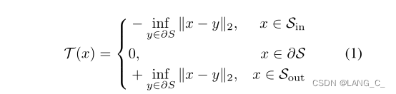
x，y代表两个不同的像素\体素，中间的那个叫做0水平集也叫做目标的轮廓， $S_{in}$ 和 $S_{out }$ 表示目标对象的内部区域和外部区域。然后定义T(x)作为从分割映射到方程中水平集函数映射的任务转换。为了将LSF任务的输出映射到分割输出的空间，自然会考虑使用T（x）的逆变换。然而，由于不可微性，在训练中整合T（x）的精确逆变换是不切实际的。因此，我们利用对水平集函数逆变换的平滑近似，前提是我们要保证在变换后的预测图中 $S_{in}$ 的值被指定为1，而 $S_{out }$ 的值被指定为0，（前景为1，背景为0）其定义为：

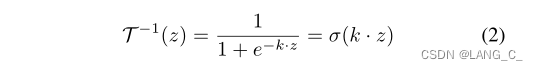
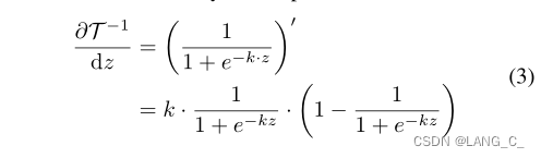
z表示像素x在水平集上的值，并且逆函数是可微的；

看一下代码如何：

def compute_sdf(img_gt, out_shape):
    """
    compute the signed distance map of binary mask
    input: segmentation, shape = (batch_size, x, y, z)
    output: the Signed Distance Map (SDM)
    sdf(x) = 0; x in segmentation boundary
             -inf|x-y|; x in segmentation
             +inf|x-y|; x out of segmentation
    normalize sdf to [-1,1]
    """

    img_gt = img_gt.astype(np.uint8)
    normalized_sdf = np.zeros(out_shape)

    for b in range(out_shape[0]):  # batch size
        posmask = img_gt[b].astype(np.bool)
        if posmask.any():
            negmask = ~posmask
            posdis = distance(posmask)
            negdis = distance(negmask)
            boundary = skimage_seg.find_boundaries(posmask, mode='inner').astype(np.uint8)
            sdf = (negdis - np.min(negdis)) / (np.max(negdis) - np.min(negdis)) - (posdis - np.min(posdis)) / (
                        np.max(posdis) - np.min(posdis))
            sdf[boundary == 1] = 0
            normalized_sdf[b] = sdf
            # assert np.min(sdf) == -1.0, print(np.min(posdis), np.max(posdis), np.min(negdis), np.max(negdis))
            # assert np.max(sdf) ==  1.0, print(np.min(posdis), np.min(negdis), np.max(posdis), np.max(negdis))

    return normalized_sdf

补充几个函数：

distance()是distance_transform_edt的使用（计算距离），计算图像中非零点到最近背景点（即0）的距离。
find_boundaries()返回标记区域之间的边界为True的bool数组

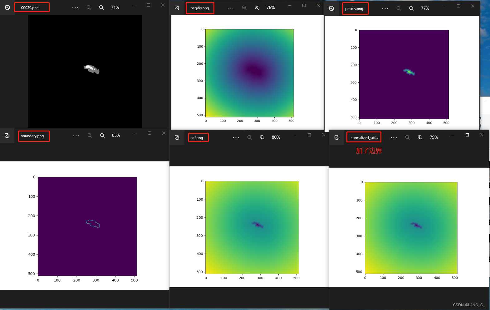
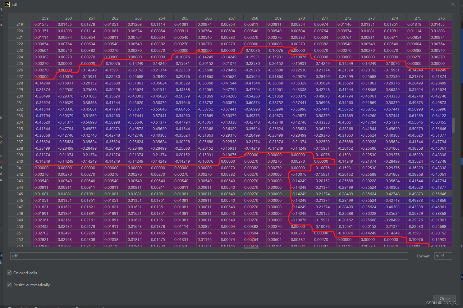
最后输出的是距离图，距离图是用来做回归使用的，这里只是加强理解。注意最后一张图的范围是（-1,1），目标域内都是负值，边界是0，背景是正值

虽然这种近似变换函数将task2的预测空间映射为与task1相同的空间，但它自然会引入任务级预测差异，因为task1侧重于像素级推理，而task2侧重于几何结构信息。因此，对于数据集D的输入X，我们定义了双任务一致性损失 $L_{DTC}$ ，以实现task1的预测 $f_{1}(x_{i})$ 和task2的预测T的转换映射之间的一致性 $T^{-1}(f_{2}(x_{i}))$

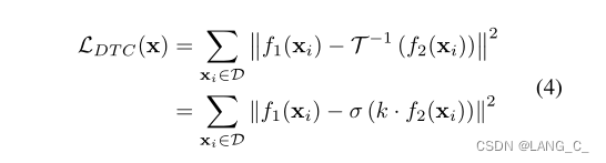
$T^{-1}(f_{2}(x_{i}))$ 的sigmoid以及一致性损失实现如下，是对outputs_tanh操作，目的是使其可微：

outputs_soft = torch.sigmoid(outputs)
...
loss_seg_dice = losses.dice_loss(
                outputs_soft[:labeled_bs, 0, :, :, :], label_batch[:labeled_bs] == 1)
dis_to_mask = torch.sigmoid(-1500*outputs_tanh)

consistency_loss = torch.mean((dis_to_mask - outputs_soft) ** 2)

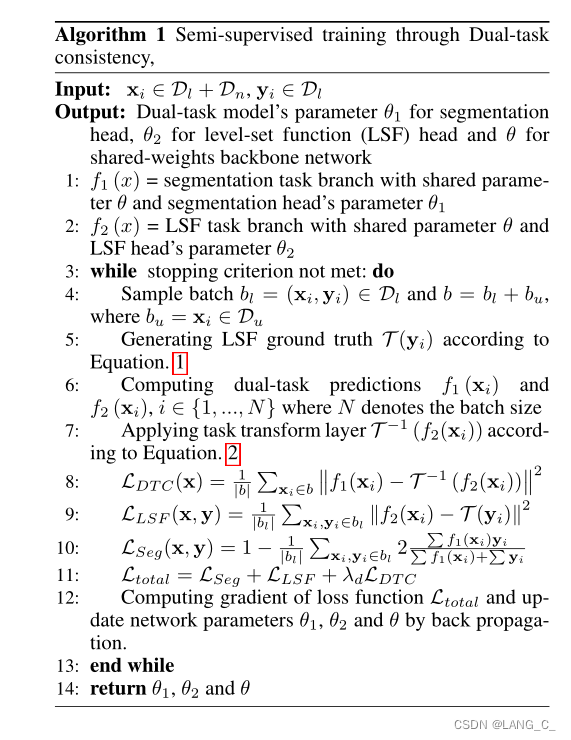
2.Semi-supervised training through Dual-Task-Consistency

分割dice损失如下：

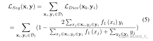
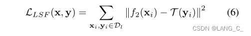
LSF的监督损失如下：

3. Algorithm

三、实验部分

数据集是100个MR左心房数据集和82个CT胰腺数据集。

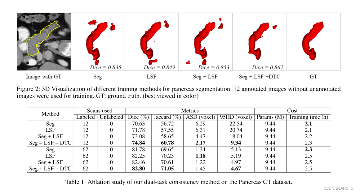
1.胰腺CT数据集上双任务一致性方法的消融研究

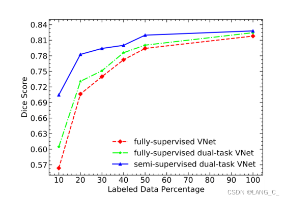
半监督学习中双任务一致性的有效性：其次，我们对我们的方法的数据利用效率进行了研究，与仅使用可用注释图像在胰腺CT数据集上进行训练的完全监督VNet和双任务VNet进行了比较。我们将结果的骰子分数绘制在图4中。可以观察到，在不同的标记数据设置中，半监督方法始终优于监督方法，这表明我们的方法有效地利用了未标记数据，并带来了性能增益。还可以发现，随着可用标记图像的增加，全监督方法和半监督方法之间的性能差距缩小，这符合常识。当标记数据数量较少时，我们的方法也可以获得比完全监督方法更好的分割结果，这表明我们提出的方法在进一步临床应用中具有很大的潜力。

2.与其他半监督方法的比较

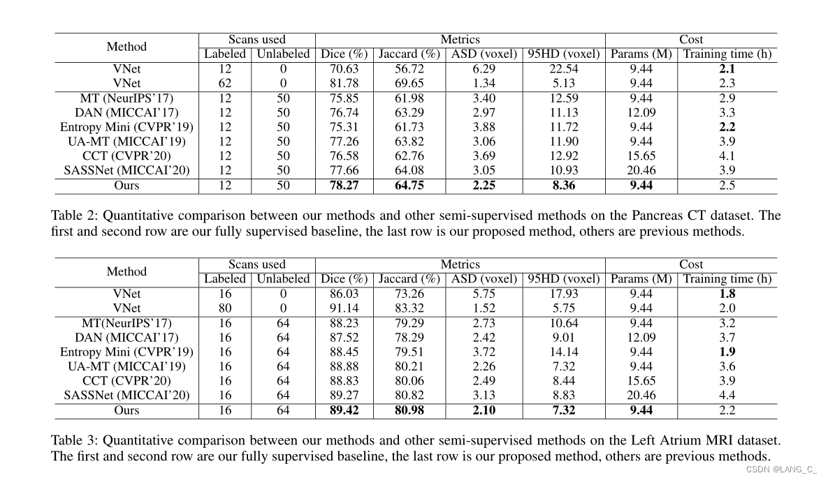
我们首先评估了我们提出的胰腺CT框架。桌子2显示了这些方法的定量比较。与仅使用12幅带注释的图像训练的全监督VNet相比，所有半监督方法都利用了未带注释的图像，显著提高了分割性能。机器翻译、UA-MT和CCT的性能略优于熵Mini和DAN，表明基于扰动的一致性损失有助于半监督分割问题。此外，UA-MT优于机器翻译，因为不确定性图可以有效地指导学生模型学习。在现有方法中，SASSNet实现了最佳性能，表明形状先验对于半监督图像分割非常有用。值得注意的是，我们的框架在所有评估指标上都比最先进的半监督方法具有更好的性能，而不需要使用复杂的多网络架构，这证实了我们的双任务一致性完全能够从未标记的数据中提取出丰富的信息。

同时，我们的框架不需要任何多重推理或迭代更新方案，这减少了计算内存成本和运行时间。

总结

在本文中，我们通过双任务一致性提出了一种新的简单的半监督医学图像分割框架，这是一种基于任务级一致性的半监督分割框架。我们使用一个双任务网络，同时预测像素级分类图和分割的水平集表示，该水平集表示能够捕获全局级形状和几何信息。为了构建半监督训练框架，我们通过任务转换层在分类图预测和LSF预测之间实现了双任务一致性。我们在两个3D医学图像数据集上获得了最新的结果，包括MR扫描中的左心房数据集和CT扫描中的胰腺数据集。优越的性能证明了我们提出的框架的有效性、鲁棒性和泛化性。在这项工作中，我们专注于单类分割以简化表示。然而，我们的方法以简单的方式扩展到多类情况。

此外，我们提出的方法可以很容易地扩展到使用额外的任务，例如边缘提取（Zhen等人。2020）和关键点估计（程等人，2020），只要两个任务之间存在可微变换。

我们还希望激励整个计算机视觉界，因为可以在多个方向上以半监督的方式构建任务一致性，例如双流视频识别（Simonyan和Zisserman 2014）、多任务图像重建（Zamir等人，2018、2020）等，以利用大量未标记的数据。未来，我们将把这种方法扩展到更多的计算机视觉应用中，以减少标记工作，并进一步研究融合策略，以集成所有不同任务的预测结果，以获得更好的性能。

测试完整代码

from matplotlib import pyplot as plt
from scipy.ndimage import distance_transform_edt as distance

import numpy as np
from PIL import Image
from skimage import segmentation as skimage_seg

def compute_sdf(img_gt, out_shape):
    """
    compute the signed distance map of binary mask
    input: segmentation, shape = (batch_size, x, y, z)
    output: the Signed Distance Map (SDM)
    sdf(x) = 0; x in segmentation boundary
             -inf|x-y|; x in segmentation
             +inf|x-y|; x out of segmentation
    normalize sdf to [-1,1]
    """

    img_gt = img_gt.astype(np.uint8)
    normalized_sdf = np.zeros(out_shape)

    for b in range(out_shape[0]):  # batch size
        posmask = img_gt[b].astype(np.bool)
        if posmask.any():
            negmask = ~posmask
            posdis = distance(posmask)
            posdis_norm = (posdis - np.min(posdis)) / (np.max(posdis) - np.min(posdis))
            negdis = distance(negmask)
            negdis_norm = (negdis - np.min(negdis)) / (np.max(negdis) - np.min(negdis))
            out = (negdis_norm + posdis_norm) * 5
            out2 = negdis + posdis
            boundary = skimage_seg.find_boundaries(posmask, mode='inner').astype(np.uint8)
            sdf = (negdis - np.min(negdis)) / (np.max(negdis) - np.min(negdis)) - (posdis - np.min(posdis)) / (
                    np.max(posdis) - np.min(posdis))
            sdf[boundary == 1] = 0
            normalized_sdf[b] = sdf
            # assert np.min(sdf) == -1.0, print(np.min(posdis), np.max(posdis), np.min(negdis), np.max(negdis))
            # assert np.max(sdf) ==  1.0, print(np.min(posdis), np.min(negdis), np.max(posdis), np.max(negdis))
            ax = plt.subplot(2, 3, 1)
            ax.set_title('Feature {}'.format(1))
            ax.axis('off')
            ax.set_title('posmask')
            plt.imshow(posmask, cmap='jet')

            ax = plt.subplot(2, 3, 2)
            ax.set_title('Feature {}'.format(2))
            ax.axis('off')
            ax.set_title('negdis')
            plt.imshow(negdis_norm, cmap='jet')

            ax = plt.subplot(2, 3, 3)
            ax.set_title('Feature {}'.format(3))
            ax.axis('off')
            ax.set_title('posdis')
            plt.imshow(posdis_norm, cmap='jet')

            ax = plt.subplot(2, 3, 4)
            ax.set_title('Feature {}'.format(4))
            ax.axis('off')
            ax.set_title('boundary')
            plt.imshow(boundary, cmap='jet')

            ax = plt.subplot(2, 3, 5)
            ax.set_title('Feature {}'.format(5))
            ax.axis('off')
            ax.set_title('out2')
            plt.imshow(out2, cmap='jet')

            ax = plt.subplot(2, 3, 6)
            ax.set_title('Feature {}'.format(6))
            ax.axis('off')
            ax.set_title('out')
            plt.imshow(out, cmap='jet')
        plt.show()  # 图像每次都不一样，是因为模型每次都需要前向传播一次，不是加载的与训练模型

    return normalized_sdf

if __name__ == '__main__':
    mask_dir = r'00024.png'
    realB_MASK = Image.open(mask_dir).convert('L')
    realB_MASK = np.array(realB_MASK)
    realB_MASK = np.expand_dims(realB_MASK, 0)
    compute_sdf(realB_MASK, realB_MASK.shape)

LANG_C_

关注

5
点赞
踩
25

收藏

觉得还不错? 一键收藏
4
评论
【论文精读】Semi-supervised Medical Image Segmentation through Dual-task Consistency

CVPR 2021 基于双任务一致性的半监督医学图像分割代码：GitHub - HiLab-git/DTC: Semi-supervised Medical Image Segmentation through Dual-task Consistency 基于深度学习的半监督学习(SSL)算法在医学图像分割方面取得了很有前景的结果，可以通过利用未标记的数据来减轻医生昂贵的注释。然而，文献中现有的SSL算法大多倾向于通过扰动网络或数据来regularize模型训练。观察到多任务/双任务学习关注具
复制链接

扫一扫