Logistic Regression实例企业还款能力评估

最新推荐文章于 2024-04-04 18:05:06 发布

Blanche117

最新推荐文章于 2024-04-04 18:05:06 发布

阅读量862

点赞数 1

分类专栏： python 文章标签：机器学习数据分析 python

本文链接：https://blog.csdn.net/weixin_45745854/article/details/113479269

版权

python 专栏收录该内容

11 篇文章

订阅专栏

本文介绍如何通过读取企业贷款数据，使用逻辑回归模型进行企业还款能力评估，通过划分训练集和测试集，并展示不同C参数下模型的召回率及混淆矩阵，探讨最优模型选择。

摘要生成于 C知道，由 DeepSeek-R1 满血版支持，前往体验 >

企业还款能力评估

步骤：

读入数据
划分训练集和测试集
训练模型
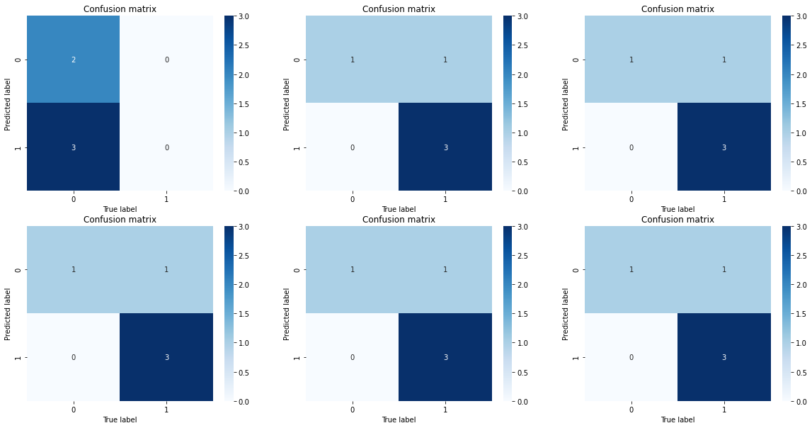
测试效果并绘制混淆矩阵

import pandas as pd
import numpy as np
import matplotlib.pyplot as plt
import seaborn as sns

%matplotlib inline

data_1 = pd.read_csv("企业贷款能力评估.csv")
print("行数：",data_1.shape[0],"列数：",data_1.shape[1])
data_1.head()

行数： 25 列数： 6

	index	x1	x2	x3
0	1	-62.8	-89.5	1.7
1	2	3.3	-3.5	1.1
2	3	-120.8	-103.2	2.5
3	4	-18.1	-28.8	1.1
4	5	-3.8	-50.6	0.9

#使用Y列不等于?的数据作为训练集
#将Y列为?的直接作为测试集
data_1.drop("index", axis=1, inplace = True)
Y_column = data_1["Y"]
#导出不含Y列的列
data_2 = data_1.loc[:,data_1.columns != "Y"]
#找出训练集和测试集的下标
indices_train = np.array(data_1[data_1.Y != "?"].index)
indices_test = np.array(data_1[data_1.Y == "?"].index)

#训练集设置
X_train = data_2.loc[indices_train,data_2.columns!="label"]
y_train = data_2.loc[indices_train,"label"]
#测试集设置
X_test = data_2.loc[indices_test,data_2.columns!="label"]
y_test = data_2.loc[indices_test,"label"]

from sklearn.linear_model import LogisticRegression
from sklearn.model_selection import KFold, cross_val_score
from sklearn.metrics import confusion_matrix, recall_score, classification_report

def plot_confusion_matrix1(cm
                          ,title='Confusion matrix'
                          ,cmap=plt.cm.Blues):
    plt.title(title)
    sns.heatmap(cm, annot=True, cmap=cmap, fmt="d")
    plt.xlabel('True label')
    plt.ylabel('Predicted label')

c_param = [0.001,0.01,0.1,1,10,100]
recall_accs=[]
j=1
plt.figure(figsize=(20,10))
for c in c_param:
    lr = LogisticRegression(C=c, penalty = "l1", solver = "liblinear")
    lr.fit(X_train, y_train.values.ravel())
    y_pred = lr.predict(X_test)
    recall_acc = recall_score(y_test, y_pred)#计算一次召回率
    print("c=",c,"时，召回率为:",recall_acc,"预测结果:",y_pred)
    #绘制混淆矩阵
    cm = confusion_matrix(y_test, y_pred)
    plt.subplot(2,3,j)
    j=j+1
    plot_confusion_matrix1(cm, title='Confusion matrix', cmap=plt.cm.Blues)
    recall_accs.append(recall_acc)

c= 0.001 时，召回率为: 0.0 预测结果: [0 0 0 0 0]
c= 0.01 时，召回率为: 1.0 预测结果: [0 1 1 1 1]
c= 0.1 时，召回率为: 1.0 预测结果: [0 1 1 1 1]
c= 1 时，召回率为: 1.0 预测结果: [0 1 1 1 1]
c= 10 时，召回率为: 1.0 预测结果: [0 1 1 1 1]
c= 100 时，召回率为: 1.0 预测结果: [0 1 1 1 1]

output_7_1