


Llama2
模型结构
1.RMSNorm
原本的Transformer中normalization一般使用层归一化。而Llama2中使用了RMSNorm=
x
M
e
a
n
(
x
2
)
+
σ
∗
γ
\frac{x}{Mean(x^2)+\sigma}*\gamma
Mean(x2)+σx∗γ。
γ
是可学习参数,
M
e
a
n
(
x
2
)
=
∑
i
=
1
N
1
N
x
i
2
\gamma是可学习参数,Mean(x^2)=\sum_{i=1}^N \frac{1}{N}x^2_i
γ是可学习参数,Mean(x2)=∑i=1NN1xi2
# RMSNorm
class RMSNorm(torch.nn.Module):
    def __init__(self, dim: int, eps: float = 1e-6):
        super().__init__()
        self.eps = eps # ε
        self.weight = nn.Parameter(torch.ones(dim)) #可学习参数γ

    def _norm(self, x):
        # RMSNorm
        return x * torch.rsqrt(x.pow(2).mean(-1, keepdim=True) + self.eps)

    def forward(self, x):
        output = self._norm(x.float()).type_as(x)
        return output * self.weight
2.RoPE
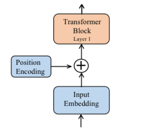
Transformer中在文本内容经过embedding层后加上一次pos_embedding就完成了加入位置信息。而Llama2中,位置编码在每个Attention层中分别对Q,K进行RoPE位置编码。也就是每次计算Attention时都要有一次位置编码。
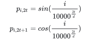
2.1 绝对位置编码
即Transformer中使用的编码方式。
2.2相对位置编码
参考:RoPE
在RoPE中,我们的出发点就是“通过绝对位置编码的方式实现相对位置编码”。
假设我们通过如下方式给q,k添加绝对位置信息
q
m
=
f
q
(
x
m
,
m
)
,
k
n
=
f
k
(
x
n
,
n
)
q_m=f_q(x_m,m),k_n=f_k(x_n,n)
qm=fq(xm,m),kn=fk(xn,n)。这样q,k就会带着m,n的位置信息。然后Attention会对他们做内积运算。我们希望通过上述函数过后,进行内积运算时能带入m-n这个相对位置信息,即
<
f
q
(
x
m
,
m
)
,
f
k
(
x
n
,
n
)
>
=
g
(
x
m
,
x
n
,
m
−
n
)
<f_q(x_m,m), f_k(x_n,n)>=g(x_m, x_n, m-n)
<fq(xm,m),fk(xn,n)>=g(xm,xn,m−n)
那么如何求解 f() 这个函数呢?有兴趣的朋友可以去看看苏神写的关于RoPE的blog[2]的求解过程部分,也可以直接去看相应的原论文RoFormer。这里直接给出答案: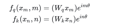
将上述带入 < f q ( x m , m ) , f k ( x n , n ) > = g ( x m , x n , m − n ) = R e [ ( W q x m ) ( W k x n ) ∗ e i ( m − n ) θ ] <f_q(x_m,m), f_k(x_n,n)>=g(x_m, x_n, m-n)=Re[(W_qx_m)(W_kx_n)^*e^{i(m-n)\theta}] <fq(xm,m),fk(xn,n)>=g(xm,xn,m−n)=Re[(Wqxm)(Wkxn)∗ei(m−n)θ]
其中 Re 表示复数的实部,
(
W
k
x
n
)
∗
(W_kx_n)^*
(Wkxn)∗ 表示
W
k
x
n
W_kx_n
Wkxn 的共轭复数。
那么现在就要考虑如何用代码实现了。
根据欧拉公式 e i x = c o s ( x ) + i s i n ( x ) e^{ix}=cos(x)+isin(x) eix=cos(x)+isin(x)带入得到 f q ( x m , m ) = ( W q x m ) [ c o s ( m θ ) + i s i n ( m θ ) ] f_q(x_m,m)=(W_qx_m)[cos(m\theta)+isin(m\theta)] fq(xm,m)=(Wqxm)[cos(mθ)+isin(mθ)]
接着论文中为了更好的利用2维平面的向量的几何性质,假设此时嵌入向量的维度为d=2
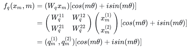
将 q m ( 1 ) , q m ( 2 ) q^{(1)}_m,q^{(2)}_m qm(1),qm(2)这个向量用复数表示 q m ( 1 ) + i q m ( 2 ) q^{(1)}_m+iq^{(2)}_m qm(1)+iqm(2)。带入展开得到
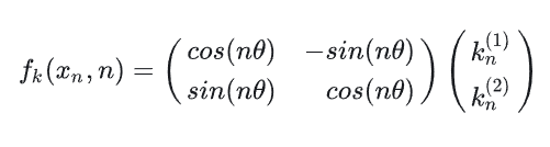
f q ( x m , m ) = [ q m ( 1 ) c o s ( m θ ) − q m ( 2 ) s i n ( m θ ) ] + i [ q m ( 1 ) s i n ( m θ ) − q m ( 2 ) c o s ( m θ ) ] f_q(x_m,m)=[q^{(1)}_mcos(m\theta)-q^{(2)}_msin(m\theta)]+i[q^{(1)}_msin(m\theta)-q^{(2)}_mcos(m\theta)] fq(xm,m)=[qm(1)cos(mθ)−qm(2)sin(mθ)]+i[qm(1)sin(mθ)−qm(2)cos(mθ)]然后将该式转换成向量表示
2.3RoPE code
def precompute_freqs_cis(dim: int, end: int, theta: float = 10000.0):
    # 计算词向量元素两两分组以后,每组元素对应的旋转角度
    # arange生成[0,2,4...126]
    freqs = 1.0 / (theta ** (torch.arange(0, dim, 2)[: (dim // 2)].float() / dim))
    # t = [0,....end]
    t = torch.arange(end, device=freqs.device)  # type: ignore
    # t为列向量 freqs为行向量做外积
    # freqs.shape = (t.len(),freqs.len()) #shape (end,dim//2)
    freqs = torch.outer(t, freqs).float()  # type: ignore
    # 生成复数
    # torch.polar(abs,angle) -> abs*cos(angle) + abs*sin(angle)*j
    freqs_cis = torch.polar(torch.ones_like(freqs), freqs)  # complex64
    # freqs_cis.shape  = (end,dim//2)
    return freqs_cis

def reshape_for_broadcast(freqs_cis: torch.Tensor, x: torch.Tensor):
    # ndim为x的维度数 ,此时应该为4
    ndim = x.ndim
    assert 0 <= 1 < ndim
    assert freqs_cis.shape == (x.shape[1], x.shape[-1])
    shape = [d if i == 1 or i == ndim - 1 else 1 for i, d in enumerate(x.shape)]
    # (1,x.shape[1],1,x.shape[-1])
    return freqs_cis.view(*shape)

def apply_rotary_emb(
    xq: torch.Tensor,
    xk: torch.Tensor,
    freqs_cis: torch.Tensor,
) -> Tuple[torch.Tensor, torch.Tensor]:
    # xq.shape = [bsz, seqlen, self.n_local_heads, self.head_dim]
    # xq_.shape = [bsz, seqlen, self.n_local_heads, self.head_dim//2 , 2]
    # torch.view_as_complex用于将二维向量转换为复数域 torch.view_as_complex即([x,y]) -> (x+yj)
    # 所以经过view_as_complex变换后xq_.shape = [bsz, seqlen, self.n_local_heads, self.head_dim//2]
    xq_ = torch.view_as_complex(xq.float().reshape(*xq.shape[:-1], -1, 2))
    xk_ = torch.view_as_complex(xk.float().reshape(*xk.shape[:-1], -1, 2))


    freqs_cis = reshape_for_broadcast(freqs_cis, xq_) # freqs_cis.shape = (1,x.shape[1],1,x.shape[-1])

    # xq_ 与freqs_cis广播哈达玛积
    # [bsz, seqlen, self.n_local_heads, self.head_dim//2] * [1,seqlen,1,self.head_dim//2]
    # torch.view_as_real用于将复数再转换回实数向量, 再经过flatten展平第4个维度
    # [bsz, seqlen, self.n_local_heads, self.head_dim//2] ->[bsz, seqlen, self.n_local_heads, self.head_dim//2,2 ] ->[bsz, seqlen, self.n_local_heads, self.head_dim]
    xq_out = torch.view_as_real(xq_ * freqs_cis).flatten(3)
    xk_out = torch.view_as_real(xk_ * freqs_cis).flatten(3)
    return xq_out.type_as(xq), xk_out.type_as(xk)
# 精简版Attention
class Attention(nn.Module):
    def __init__(self, args: ModelArgs):
        super().__init__()
        self.wq = Linear(...)
        self.wk = Linear(...)
        self.wv = Linear(...)

        self.freqs_cis = precompute_freqs_cis(dim, max_seq_len * 2)

    def forward(self, x: torch.Tensor):
        bsz, seqlen, _ = x.shape
        xq, xk, xv = self.wq(x), self.wk(x), self.wv(x)
        xq = xq.view(bsz, seqlen, self.n_local_heads, self.head_dim)
        xk = xk.view(bsz, seqlen, self.n_local_kv_heads, self.head_dim)
        xv = xv.view(bsz, seqlen, self.n_local_kv_heads, self.head_dim)
         # attention 操作之前,应用旋转位置编码
        xq, xk = apply_rotary_emb(xq, xk, freqs_cis=freqs_cis)
        #...
        # 进行后续Attention计算
        scores = torch.matmul(xq, xk.transpose(1, 2)) / math.sqrt(dim)
        scores = F.softmax(scores.float(), dim=-1)
        output = torch.matmul(scores, xv)  # (batch_size, seq_len, dim)
  # ......
3.KV Cache and GQA
3.1 KV Cache
大模型推理性能优化的一个常用技术是KV Cache。由于我们生成时,是自回归生成,
T
t
−
1
T_{t-1}
Tt−1时刻生成了1-2-3,同时也生成了
K
t
−
1
,
V
t
−
1
K_{t-1},V_{t-1}
Kt−1,Vt−1。在
T
t
T_t
Tt时刻生成1-2-3-4,此时难道我们还需要完全重新计算一次
K
t
,
V
t
K_t,V_t
Kt,Vt吗?当然不是。
在 T t − 1 T_{t-1} Tt−1时刻后,我们可以把Q完全丢弃,然后将 K t − 1 , V t − 1 K_{t-1},V_{t-1} Kt−1,Vt−1存入缓存。然后 T t T_t Tt时刻,我们会有 Q 1 − 2 − 3 − 4 Q_{1-2-3-4} Q1−2−3−4,拿这个 Q 4 Q_4 Q4和 K t − 1 K_{t-1} Kt−1内积,就可以得到新的 K t K_t Kt了。
def forward(
        self,
        x: torch.Tensor,
        start_pos: int,
        freqs_cis: torch.Tensor,
        mask: Optional[torch.Tensor],
    ):
        bsz, seqlen, _ = x.shape
        xq, xk, xv = self.wq(x), self.wk(x), self.wv(x)

        xq = xq.view(bsz, seqlen, self.n_local_heads, self.head_dim)
        xk = xk.view(bsz, seqlen, self.n_local_kv_heads, self.head_dim)
        xv = xv.view(bsz, seqlen, self.n_local_kv_heads, self.head_dim)

        xq, xk = apply_rotary_emb(xq, xk, freqs_cis=freqs_cis) #嵌入RoPE位置编码
        # 设备转换
        self.cache_k = self.cache_k.to(xq)
        self.cache_v = self.cache_v.to(xq)

        # 按此时序列的句子长度把kv添加到cache中
        # 初始在prompt阶段seqlen>=1, 后续生成过程中seqlen==1
        self.cache_k[:bsz, start_pos : start_pos + seqlen] = xk
        self.cache_v[:bsz, start_pos : start_pos + seqlen] = xv

        # 读取新进来的token所计算得到的k和v
        keys = self.cache_k[:bsz, : start_pos + seqlen]
        values = self.cache_v[:bsz, : start_pos + seqlen]

        # repeat k/v heads if n_kv_heads < n_heads
        keys = repeat_kv(keys, self.n_rep)  # (bs, seqlen, n_local_heads, head_dim)
        values = repeat_kv(values, self.n_rep)  # (bs, seqlen, n_local_heads, head_dim)

        xq = xq.transpose(1, 2)  # (bs, n_local_heads, seqlen, head_dim)
        keys = keys.transpose(1, 2)
        values = values.transpose(1, 2)
3.2 MQA & GQA
即使这样,我们也还是存不下,假设Llama2-7b模型,embedding-dim=4096。使用float16数据类型。那么在一个TransformerBlock中就需要占用
4096
∗
2
∗
2
=
16
k
b
4096*2*2=16kb
4096∗2∗2=16kb,而模型一共32个Block
16
∗
32
=
512
k
b
16*32=512kb
16∗32=512kb,那么如果我们的输入数据长度是1024的话…
所以我们还需要减少存储的内容,那么请看下图
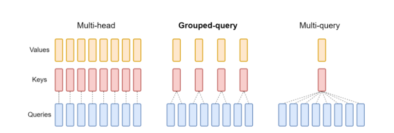
很直观,也就是多头注意力中,我们将原来一个Q对应一个KV的结构变成了2个Q对应一个KV或者所有Q对应一个KV。


 4539
4539


 被折叠的 条评论
为什么被折叠?
被折叠的 条评论
为什么被折叠?
 到【灌水乐园】发言


