


文章目录
前言
笔者权当做笔记,借鉴的是《Python 深度学习》这本书,里面的代码也都是书上的代码,用的是jupyter notebook 编写代码后期用的pycharm编写。今天开始用卷积神经网络作用于“猫狗数据集”。本人认为这一节非常重要,《Python 深度学习》这本书上讲的也非常详细,本人也是琢磨了好久。记录一下勉励自己在这条路上坚持地走下去!🙂
1.下载数据集
“猫狗分类数据集”不是内置在keras中。《Python 深度学习》这本书用到的是Kaggle上的数据集。整个数据集包含25 000张猫狗图像(每个类别包含12 500张),大小为543MB(压缩后);这里我们根据这个我们创建一个小型的数据集,每个类别各1000个样本的训练集、每个类别各500个验证集和500个测试集。这里方便大家,贴出了文章需要的数据集:需要用到的数据集
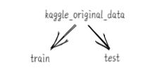
train文件下的图像]

test目录下的图像

2.创建小型数据集
将图像复制到训练、验证和测试的目录
import os, shutil

original_dataset_dir = 'E:/mydata/catsanddog/kaggle_original_data/train'  # 原始的数据集的训练集
base_dir = 'E:/mydata/catsanddog/cats_and_dogs_small'
os.mkdir(base_dir)  # 创建一个较小数据集的目录

# 创建训练验证和测试的目录
train_dir = os.path.join(base_dir, 'train')
os.mkdir(train_dir)
validation_dir = os.path.join(base_dir, 'validation')
os.mkdir(validation_dir)
test_dir = os.path.join(base_dir, 'test')
os.mkdir(test_dir)

# 创建猫狗训练验证和测试的目录
train_cats_dir = os.path.join(train_dir, 'cats')
os.mkdir(train_cats_dir)
train_dogs_dir = os.path.join(train_dir, 'dogs')
os.mkdir(train_dogs_dir)

validation_cats_dir = os.path.join(validation_dir, 'cats')
os.mkdir(validation_cats_dir)
validation_dogs_dir = os.path.join(validation_dir, 'dogs')
os.mkdir(validation_dogs_dir)

test_cats_dir = os.path.join(test_dir, 'cats')
os.mkdir(test_cats_dir)
test_dogs_dir = os.path.join(test_dir, 'dogs')
os.mkdir(test_dogs_dir)

# 复制猫猫的图像
# 将前1000张猫的图像复制到train_cats_dir
fnames = ['cat.{}.jpg'.format(i) for i in range(1000)]
for fname in fnames:
    src = os.path.join(original_dataset_dir, fname)
    dst = os.path.join(train_cats_dir, fname)
    shutil.copyfile(src, dst)

# 将剩下的500张猫的图像复制到validation_cats_dir
fnames = ['cat.{}.jpg'.format(i) for i in range(1000, 1500)]
for fname in fnames:
    src = os.path.join(original_dataset_dir, fname)
    dst = os.path.join(validation_cats_dir, fname)
    shutil.copyfile(src, dst)

# 将剩下500张猫的图像复制到test_cats_dir
fnames = ['cat.{}.jpg'.format(i) for i in range(1500, 2000)]
for fname in fnames:
    src = os.path.join(original_dataset_dir, fname)
    dst = os.path.join(test_cats_dir, fname)
    shutil.copyfile(src, dst)


# 复制狗狗的图像
# 将前1000张狗的图像复制到train_dogs_dir
fnames = ['dog.{}.jpg'.format(i) for i in range(1000)]
for fname in fnames:
    src = os.path.join(original_dataset_dir, fname)
    dst = os.path.join(train_dogs_dir, fname)
    shutil.copyfile(src, dst)

# 将剩下的500张狗的图像复制到validation_dogs_dir
fnames = ['dog.{}.jpg'.format(i) for i in range(1000, 1500)]
for fname in fnames:
    src = os.path.join(original_dataset_dir, fname)
    dst = os.path.join(validation_dogs_dir, fname)
    shutil.copyfile(src, dst)

# 将剩下500张狗的图像复制到test_dogs_dir
fnames = ['dog.{}.jpg'.format(i) for i in range(1500, 2000)]
for fname in fnames:
    src = os.path.join(original_dataset_dir, fname)
    dst = os.path.join(test_dogs_dir, fname)
    shutil.copyfile(src, dst)
# 检查一下每一个分组中包含多少张图像
print('训练猫图像:', len(os.listdir(train_cats_dir)))
print('训练狗图像:', len(os.listdir(train_dogs_dir)))
print('验证猫图像:', len(os.listdir(validation_cats_dir)))
print('验证狗图像:', len(os.listdir(validation_dogs_dir)))
print('测试猫图像:', len(os.listdir(test_cats_dir)))
print('测试狗图像:', len(os.listdir(test_dogs_dir)))
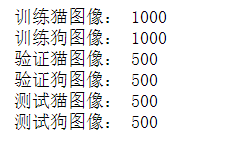
总计:2000 张训练图像、1000张验证图像和1000张测试图像。
3.构建网络
这本书上使用的是:初始输入的尺寸为150 * 150,最后在Flatten层之前的特征图大小为7 * 7.
注意: 网络中特征图的深度在逐渐增大(从32增大到128),而特征图的尺寸在逐渐减小从150 * 150 减小到 7 * 7 这几乎是所有卷积神经网络的模式。
我们面临的是一个二分问题,所以最后一层使用sigmoid激活的单一单元(大小为1的Dense层)。这个单元将对某个类别的概率进行编码。
将猫狗分类的小型卷积神经网络实例化
import keras
from keras import layers, models
from keras import optimizers, losses

model = models.Sequential()

model.add(layers.Conv2D(32, (3, 3), activation='relu', input_shape=(150, 150, 3)))
model.add(layers.MaxPooling2D((2, 2)))
model.add(layers.Conv2D(64, (3, 3), activation='relu'))
model.add(layers.MaxPooling2D((2, 2)))
model.add(layers.Conv2D(128, (3, 3), activation='relu'))
model.add(layers.MaxPooling2D((2, 2)))
model.add(layers.Conv2D(128, (3, 3), activation='relu'))
model.add(layers.MaxPooling2D((2, 2)))
model.add(layers.Flatten())
model.add(layers.Dense(512, activation='relu'))
model.add(layers.Dense(1, activation='sigmoid'))
# 在编译之前可以查看网络的架构
model.summary()

# 编译模型
# model.compile(loss=losses.binary_crossentropy, optimizer=optimizers.RMSprop(lr=1e-4), metrics=['acc'])  # 这个是书上的,指定了学习率
model.compile(loss=losses.binary_crossentropy, optimizer='rmsprop', metrics=['acc'])
4.数据预处理
数据输入神经网络之前,数据格式化为经过预处理的浮点数张量。
	1、读取图像文件
	2、将JPEG文件解码为RGB像素网格
	3、将这些像素网格转换为浮点数张量
	4、将像素值(0~255范围内)缩放到[0-1]区间
keras可以自动完成这些步骤!
# keras.preprocessing.image图像处理辅助工具模块
from keras.preprocessing.image import ImageDataGenerator

train_datagen = ImageDataGenerator(rescale=1./255)
test_datagen = ImageDataGenerator(rescale=1./255)

train_generator = train_datagen.flow_from_directory(train_dir, target_size=(150, 150), batch_size=20, class_mode='binary')
validation_generator = train_datagen.flow_from_directory(validation_dir, target_size=(150, 150), batch_size=20, class_mode='binary')
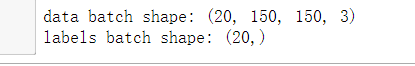
# 可以看一下其中一个生成器的输出,生成的是150 * 150 的RGB图像(形状为(20, 150, 150, 3))与二进制标签(形状为(20, ))组成的批量。
for data_batch, labels_batch in train_generator:
    print('data batch shape:', data_batch.shape)
    print('labels batch shape:', labels_batch.shape)
    break
5.训练模型
# 利用批量生成器拟合模型
h = model.fit_generator(train_generator, steps_per_epoch=100, epochs=30, validation_data=validation_generator,validation_steps=50)
预计是15分钟,建议刷一道数学题🙂
训练过程

保存模型
model.save('cats_and_dogs_small_1.h5') # 保存模型
6.绘制图像(损失率和精度)
# 绘制损失曲线和精度曲线
# 绘制损失曲线和精度曲线
import matplotlib.pyplot as plt

acc = h.history.get('acc')
val_acc = h.history.get('val_acc')
loss = h.history.get('loss')
val_loss = h.history.get('val_loss')

epochs = range(1, len(acc) + 1)

plt.xlabel('epochs')
plt.ylabel('percentage')
plt.plot(epochs, acc, 'r', label='Training acc')
plt.plot(epochs, val_acc, 'b', label='Validation acc')
plt.title('Training and validation accuracy')
plt.legend()

plt.figure()

plt.xlabel('epochs')
plt.ylabel('percentage')
plt.plot(epochs, loss, 'r', label='Training loss')
plt.plot(epochs, val_loss, 'b', label='Validation loss')
plt.title('Training and validation loss')
plt.legend()

plt.show()
准确率图像

损失率图像

7.分析结果
从这些图像中能看到“过拟合”的特征。
训练的精度随证轮次的增加,逐渐增加,趋于100%,然而验证的精度一直滞留在70%左右。
验证的损失起伏太大,训练的损失一直递减。
**需要一种新的方法处理图像**,那就是数据增强!
8.数据增强
过拟合原因是因为学习样本太少,导致无法训练出能够泛化到新数据的模型。
如果拥有无限的数据,那么模型能够观察到数据分布的所有内容,这样永远不会过拟合。
数据增强是从现有的训练样本中生成更多的训练数据,其方法就是利用多种能够生成可信图像的随机变换来增加样本。
目标就是:模型在训练时不会两次查看完全相同的图像。这样模型观察到的数据更多,从而具有更好的泛化能力。
datagen = ImageDataGenerator(rotation_range=40,  # 角度值(0-180)表示图像随机旋转的范围
                             width_shift_range=0.2,  # 水平向上平移的范围(相对于总宽度的比例)
                             height_shift_range=0.2, # 垂直向上平移的范围(相对于总高度的比例)
                             shear_range=0.2,  # 随机错切变换的角度
                             zoom_range=0.2,   # 随机缩放的范围
                             horizontal_flip=True,  # 随机将图像水平翻转
                             fill_mode='nearest')  # 用于填充新创建像素的方法,可能来自于旋转或宽度/高度平移
# 书上的代码展示的图像是垂直的
from keras.preprocessing import image
fnames = [os.path.join(train_cats_dir, fname) for fname in os.listdir(train_cats_dir)]

img_path = fnames[3]  # 选择一张图像进行增强
img = image.load_img(img_path, target_size=(150, 150))  # 读取图像并调整大小
x= image.img_to_array(img)  # 将其转换为形状(150, 150, 3)的Numpy数组
x = x.reshape((1, ) + x.shape)  # 将其转换为形状(1, 150, 150, 3)

i = 0
for batch in datagen.flow(x, batch_size=1):
    plt.figure(i)
    imgplot = plt.imshow(image.array_to_img(batch[0]))
    i += 1
    if i % 4 == 0:  # 生成随机变换后的图像批量。循环无限,所以需要在某个时刻终止循环
        break

plt.show()

# 水平展示子图
# 这样好看一点
fnames = [os.path.join(train_cats_dir, fname) for fname in os.listdir(train_cats_dir)]

img_path = fnames[3]  # 选择一张图像进行增强
img = image.load_img(img_path, target_size=(150, 150))  # 读取图像并调整大小
x= image.img_to_array(img)  # 将其转换为形状(150, 150, 3)的Numpy数组
x = x.reshape((1, ) + x.shape)  # 将其转换为形状(1, 150, 150, 3)

i = 0
ans = 221
for batch in datagen.flow(x, batch_size=1):
    plt.subplot(ans)
    plt.imshow(image.array_to_img(batch[0]))
    i += 1
    ans += 1
    if i % 4 == 0:  # 生成随机变换后的图像批量。循环无限,所以需要在某个时刻终止循环
        break

plt.show()

小结
如果使用这种数据增强来训练一个新网络,那么网络将不会两次看到同样的输入。但是网络看到的输入仍然是高度相关的,这些输入都来自于少量的原始图像。我们无法生成新信息,只能混合现有信息。所以这种方法可能不能不足以完全消除过拟合。为了进一步降低过拟合,需要向模型中添加一个Dropout层,添加到密集连接分类器之前。
9.包含dropout层的新卷积神经网络
model = models.Sequential()
model.add(layers.Conv2D(32, (3, 3), activation='relu', input_shape=(150, 150, 3)))
model.add(layers.MaxPooling2D((2, 2)))
model.add(layers.Conv2D(64, (3, 3), activation='relu'))
model.add(layers.MaxPooling2D((2, 2)))
model.add(layers.Conv2D(128, (3, 3), activation='relu'))
model.add(layers.MaxPooling2D((2, 2)))
model.add(layers.Conv2D(128, (3, 3), activation='relu'))
model.add(layers.MaxPooling2D((2, 2)))
model.add(layers.Flatten())
model.add(layers.Dropout(0.5))
model.add(layers.Dense(512, activation='relu'))
model.add(layers.Dense(1, activation='sigmoid'))

model.compile(loss='binary_crossentropy', optimizer='rmsprop', metrics=['accuracy'])
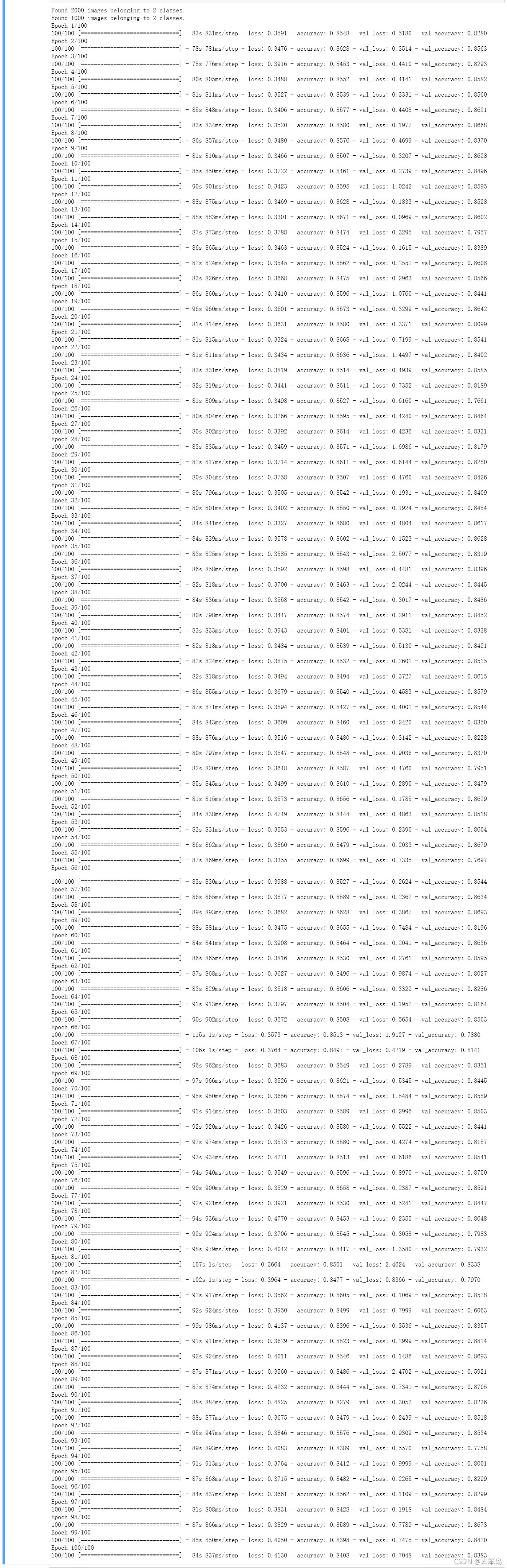
10.训练这个包含dropout层的新卷积神经网络
注意: 这里训练的时间会稍微长一些,建议干一些其他的事请(我这里去吃了一顿饭回来发现还没有训练完,最后发现代码写错了,无奈又训练了一遍/(ㄒoㄒ)/~~);应该是2个小时多一点,在jupyter notebook上跑的。
train_datagen = ImageDataGenerator(rescale=1./255,
                                   rotation_range=40,
                                   width_shift_range=0.2,
                                   height_shift_range=0.2,
                                   shear_range=0.2,
                                   zoom_range=0.2,
                                   horizontal_flip=True, )
test_datagen = ImageDataGenerator(rescale=1./255)
# 不能增强验证数据

train_generator = train_datagen.flow_from_directory(train_dir,
                                                    target_size=(150, 150),
                                                    batch_size=32,
                                                    class_mode='binary')

validation_generator = test_datagen.flow_from_directory(validation_dir,
                                                    target_size=(150, 150),
                                                    batch_size=32,
                                                    class_mode='binary')

h = model.fit_generator(train_generator,
                        steps_per_epoch=100,
                        epochs=100,
                        validation_data=validation_generator,
                        validation_steps=50)
保存模型
# 保存模型
model.save('cats_and_dogs_small_2.h5')
11.绘制这个包含dropout层的新卷积神经网络模型的损失率和准确率图像
# 绘制损失曲线和精度曲线
import matplotlib.pyplot as plt

acc = h.history.get('accuracy')
val_acc = h.history.get('val_accuracy')
loss = h.history.get('loss')
val_loss = h.history.get('val_loss')

epochs = range(1, len(acc) + 1)

plt.xlabel('epochs')
plt.ylabel('percentage')
plt.plot(epochs, acc, 'r', label='Training acc')
plt.plot(epochs, val_acc, 'b', label='Validation acc')
plt.title('Training and validation accuracy')
plt.legend()

plt.figure()

plt.xlabel('epochs')
plt.ylabel('percentage')
plt.plot(epochs, loss, 'r', label='Training loss')
plt.plot(epochs, val_loss, 'b', label='Validation loss')
plt.title('Training and validation loss')
plt.legend()

plt.show()
**可以看出:**精度提高了不少。

12.使用预训练的卷积神经网络
预训练卷积神经网络是一个保存好的网络,之前已在大型数据集(通常是大规模图像分类任务)上训练好。我们这里使用VGG16架构,它是一种简单而又广泛使用的卷积神经网络。
使用预训练网络有两种方法:特征提取和微调模型。
from keras.applications import VGG16
import os

'''
weights='imagenet',  模型初始化的权重检查点
include_top=False,   指定模型最后是否包含密集连接分类器。
默认情况下,这个密集连接分类器对应于ImageNet的1000个类别。这里我们使用的就是两个类别(cats and dogs)
input_shape=(150, 150, 3)  输入到网络中的图像张量形状。
'''

conv_base = VGG16(weights='imagenet',
                  include_top=False,
                  input_shape=(150, 150, 3))

print(conv_base.summary())
**这里有一个问题:**如果是直接加载的vgg16模型,没有梯子的话,按照书上的那种会报错,导致模型无法加载。
编译器会弹出从这个链接下载
下载完毕后,权重改为下载的路径即可加载vgg16模型;之后再次运行书中的代码就变得非常的快!
from keras.applications import VGG16
import os

'''
weights='imagenet',  模型初始化的权重检查点
include_top=False,   指定模型最后是否包含密集连接分类器。
默认情况下,这个密集连接分类器对应于ImageNet的1000个类别。这里我们使用的就是两个类别(cats and dogs)
input_shape=(150, 150, 3)  输入到网络中的图像张量形状。
'''
path = "../mydatas/vgg16_weights_tf_dim_ordering_tf_kernels_notop (1).h5"
conv_base = VGG16(weights=path,
                  include_top=False,
                  input_shape=(150, 150, 3))

print(conv_base.summary())

再次使用书中的代码就会很快地加载。
我们可以使用python里面的工具保存一下架构图(需要pip install graphviz)。
from keras.applications import VGG16
import os

'''
weights='imagenet',  模型初始化的权重检查点
include_top=False,   指定模型最后是否包含密集连接分类器。
默认情况下,这个密集连接分类器对应于ImageNet的1000个类别。这里我们使用的就是两个类别(cats and dogs)
input_shape=(150, 150, 3)  输入到网络中的图像张量形状。
'''
# path = "../mydatas/vgg16_weights_tf_dim_ordering_tf_kernels_notop (1).h5"

conv_base = VGG16(weights='imagenet',
                  include_top=False,
                  input_shape=(150, 150, 3))

print(conv_base.summary())

from keras.utils import plot_model
plot_model(conv_base, show_shapes=True, to_file='VGG16.png')

from IPython.display import Image
Image(filename='VGG16.png')

这里我换成了pycharm来跑代码。

from keras.applications import VGG16
import os

'''
weights='imagenet',  模型初始化的权重检查点
include_top=False,   指定模型最后是否包含密集连接分类器。
默认情况下,这个密集连接分类器对应于ImageNet的1000个类别。这里我们使用的就是两个类别(cats and dogs)
input_shape=(150, 150, 3)  输入到网络中的图像张量形状。
'''
# path = "../mydatas/vgg16_weights_tf_dim_ordering_tf_kernels_notop (1).h5"

conv_base = VGG16(weights='imagenet',
                  include_top=False,
                  input_shape=(150, 150, 3))

print(conv_base.summary())

最后特征图形状为(4, 4, 512)。需要在这个特征上添加一个密集连接分类器。
两种方法可供选择。
一:在数据集上运行卷积基,将输出保存成硬盘中的Numpy数组,然后用这个数组作为输入,
		输入到独立的密集连接分类器中;这种方法速度快,计算代价低,因为对每个输入图像只需运行
		一次卷积基,(而卷积基是目前流程中计算代价最高的,这种方法不允许使用“数据增强”)

二:在顶部添加Dense层来扩展已有的模型,并在输入数据上端到端地运行整个模型,
       这样可以使用“数据增强”(因为每个输入图像进入模型都会经过卷积基,但是这种代价要很高)
1.不使用数据增强地快速特征提取

# 方法一:不使用数据增强地快速特征提取
# import tensorflow as tf
# if __name__ == '__main__':
#     print(tf.__version__)
#     if tf.test.gpu_device_name():
#         print('Default GPU Device: {}'.format(tf.test.gpu_device_name()))
#     else:
#         print("Please install GPU version of TF")


# 使用预训练的卷积基提取特征
import os
import instantiation
import numpy as np
from keras.preprocessing.image import ImageDataGenerator

base_dir = "E://mydata//catsanddog//cats_and_dogs_small"
# base_dir = 1
print(base_dir)
train_dir = os.path.join(base_dir, 'train')
validation_dir = os.path.join(base_dir, 'validation')
test_dir = os.path.join(base_dir, 'test')

datagen = ImageDataGenerator(rescale=1./255)
batch_size = 20


def extract_features(directory, sample_count):
    features = np.zeros(shape=(sample_count, 4, 4, 512))
    labels = np.zeros(shape=(sample_count))
    generator = datagen.flow_from_directory(
        directory,
        target_size=(150, 150),
        batch_size=batch_size,
        class_mode='binary'
    )
    i = 0
    for inputs_batch, lables_batch in generator:
        features_bath = instantiation.conv_base.predict(inputs_batch)
        features[i * batch_size : (i + 1) * batch_size] = features_bath
        labels[i * batch_size : (i + 1) * batch_size] = lables_batch
        i += 1
        if i * batch_size >= sample_count:
            break
    return features, labels


train_features, train_labels = extract_features(train_dir, 2000)
validation_features, validation_labels = extract_features(validation_dir, 1000)
test_features, test_labels = extract_features(test_dir, 1000)

# 展平
train_features = np.reshape(train_features, (2000, 4 * 4 * 512))
validation_features = np.reshape(validation_features, (1000, 4 * 4 * 512))
test_features = np.reshape(test_features, (1000, 4 * 4 * 512))

# 定义并训练密集连接分类器

from keras import models
from keras import layers
from keras import optimizers
import not_quick_extract as m_one

model = models.Sequential()
model.add(layers.Dense(256, activation='relu', input_dim=4 * 4 * 512))
model.add(layers.Dropout(0.5))
model.add(layers.Dense(1, activation='sigmoid'))

model.compile(optimizer='rmsprop',
              loss='binary_crossentropy',
              metrics=['acc'])

h = model.fit(m_one.train_features, m_one.train_labels,
              epochs=30,
              batch_size=20,
              validation_data=(m_one.validation_features, m_one.validation_labels))

# 绘制损失率和准确率图像
import matplotlib.pyplot as plt
import one_method_fit as F

acc = F.h.history.get('acc')
val_acc = F.h.history.get('val_acc')
loss = F.h.history.get('loss')
val_loss = F.h.history.get('val_loss')

epochs = range(1, len(acc) + 1)

plt.plot(epochs, acc, 'r', label='Training acc')
plt.plot(epochs, val_acc, 'b', label='Validation acc')
plt.title('Training and validation accuracy')
plt.xlabel('epochs')
plt.ylabel('per')
plt.legend()

plt.figure()

plt.plot(epochs, loss, 'r', label='Training loss')
plt.plot(epochs, val_loss, 'b', label='Validation loss')
plt.title('Training and validation loss')
plt.xlabel('epochs')
plt.ylabel('per')
plt.legend()

plt.show()
运行结果

准确率图像

损失率图像

小结:验证的精度明显达到了90%,但是模型从一开始就出现“过拟合”的现象。因为这个方法没用到“数据增强”。
	 而“数据增强”对小型的数据集的“过拟合”特别重要!
2.使用数据增强的特征提取
本方法计算代价很高,保证电脑能用GPU跑模型。
import instantiation as My  # 导入conv_base
from keras import models
from keras import layers

model = models.Sequential()
model.add(My.conv_base)  # 添加conv_base
model.add(layers.Flatten())
model.add(layers.Dense(256, activation='relu'))
model.add(layers.Dense(1, activation='sigmoid'))

但是VGG16的卷积基有14,714,688个参数,太多啦。所以我们需要采取“冻结”卷积基。(在编译和训练模型之前)
冻结一个或多个层是指在训练过程中保持其权重不变。如果不这样做,那么    卷积基之前学到的表示将会在网络中被修改,因为其上的Dense层是随机初始化的,所以非常大的权重更新将会在网络中传播,对之前学到的表示造成很大的破坏。
import instantiation as My
from keras import models
from keras import layers

model = models.Sequential()
model.add(My.conv_base)
model.add(layers.Flatten())
model.add(layers.Dense(256, activation='relu'))
model.add(layers.Dense(1, activation='sigmoid'))

print('This is ths number of trainable weights '
      'before freezing ths conv base:', len(model.trainable_weights))

My.conv_base.trainable = False  # 设置就是把trainable设置为False即可

print('This is ths number of trainable weights '
      'before freezing ths conv base:', len(model.trainable_weights))


# 利用冻结的卷积基端到端地训练模型
import os
from keras.preprocessing.image import ImageDataGenerator
from keras import optimizers
import my_add as my


base_dir = "E://mydata//catsanddog//cats_and_dogs_small"
# base_dir = 1
print(base_dir)
train_dir = os.path.join(base_dir, 'train')
validation_dir = os.path.join(base_dir, 'validation')
test_dir = os.path.join(base_dir, 'test')

train_datagen = ImageDataGenerator(
    rescale=1./255,
    rotation_range=40,
    width_shift_range=0.2,
    height_shift_range=0.2,
    shear_range=0.2,
    zoom_range=0.2,
    horizontal_flip=True,
    fill_mode='nearest'

)

test_datagen = ImageDataGenerator(rescale=1./255)

train_generator = train_datagen.flow_from_directory(
    train_dir,
    target_size=(150, 150),
    batch_size=20,
    class_mode='binary'
)

validation_generator = test_datagen.flow_from_directory(
    validation_dir,
    target_size=(150, 150),
    batch_size=20,
    class_mode='binary'
)

my.model.compile(loss='binary_crossentropy',
                 # optimizer=optimizers.RMSprop(lr=2e-5),
                 optimizer='rmsprop',
                 metrics=['acc'])

h = my.model.fit_generator(
    train_generator,
    steps_per_epoch=100,
    epochs=30,
    validation_data=validation_generator,
    validation_steps=50
)
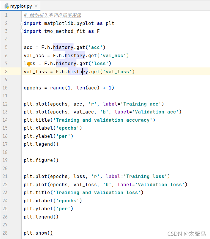
# 绘制损失率和准确率图像
import matplotlib.pyplot as plt
import two_method_fit as F

acc = F.h.history.get('acc')
val_acc = F.h.history.get('val_acc')
loss = F.h.history.get('loss')
val_loss = F.h.history.get('val_loss')

epochs = range(1, len(acc) + 1)

plt.plot(epochs, acc, 'r', label='Training acc')
plt.plot(epochs, val_acc, 'b', label='Validation acc')
plt.title('Training and validation accuracy')
plt.xlabel('epochs')
plt.ylabel('per')
plt.legend()

plt.figure()

plt.plot(epochs, loss, 'r', label='Training loss')
plt.plot(epochs, val_loss, 'b', label='Validation loss')
plt.title('Training and validation loss')
plt.xlabel('epochs')
plt.ylabel('per')
plt.legend()

plt.show()
运行结果

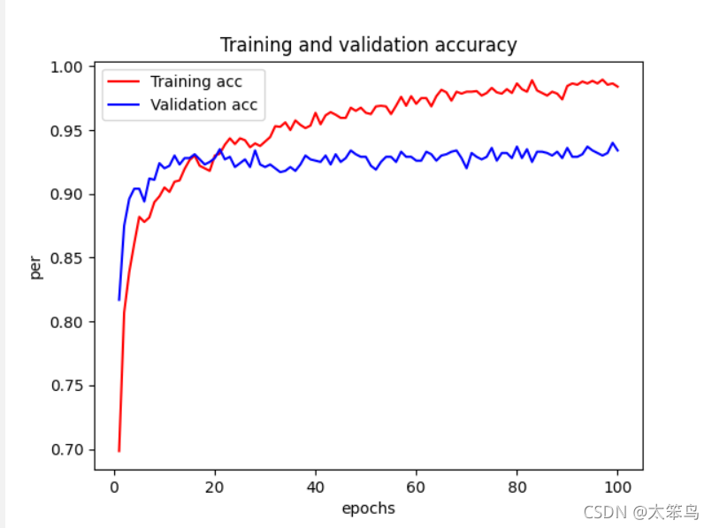
准确率图像

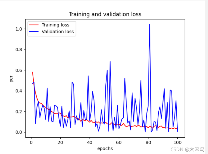
损失率图像

这里我的验证的准确率还是90%左右,没有到达书上的96%,但是很明显的看出”过拟合“现象避免的很好啦。
13.微调模型
模型微调,与特征提取互为补充。对于用于特征提取的冻结的模型基,微调是指将其顶部的几层“解冻”,并将这解冻的几层和新增加的部分
(全连接分类器)联合训练。微调:略微调整了所复用模型中更加抽象的表示,以便让这些表示与手头的问题更加相关。

冻结VGG16的卷积基是为了能够在上面训练一个随机初始化的分类器。只有上面的分类器训练好了,才能微调卷积基的顶部几层;如果分类
器没有训练好,那么训练期间通过网络传播的误差信号会特别大,微调几层之前学到的表示都会被破坏。


微调网络的步骤:
	1、在已经训练好的基网络上调价自定义网络;
	2、冻结基网络;
	3、训练所添加的部分;
	4、解冻基网络的一些层;
	5、联合训练解冻的这些层和添加的部分
**注意:**微调更靠底部的层,得到的回报会更少;训练的参数越多,过拟合风险越大。卷积基有1500万个参数,在小型数据集上训练这么多参数是有风险的。
# 模型微调
from keras.applications import VGG16
from keras import models, optimizers
from keras import layers
from keras.preprocessing.image import ImageDataGenerator
import os
import matplotlib.pyplot as plt


'''
weights='imagenet',  模型初始化的权重检查点
include_top=False,   指定模型最后是否包含密集连接分类器。
默认情况下,这个密集连接分类器对应于ImageNet的1000个类别。这里我们使用的就是两个类别(cats and dogs)
input_shape=(150, 150, 3)  输入到网络中的图像张量形状。
'''
# path = "../mydatas/vgg16_weights_tf_dim_ordering_tf_kernels_notop (1).h5"

conv_base = VGG16(weights='imagenet',
                  include_top=False,
                  input_shape=(150, 150, 3))

model = models.Sequential()
model.add(conv_base)
model.add(layers.Flatten())
model.add(layers.Dense(256, activation='relu'))
model.add(layers.Dense(1, activation='sigmoid'))
print(conv_base.summary())


'''
调整最后三个卷积层,就是直到block4_pool的所有层都应该被冻结,
                而block5_conv1、block5_conv2和block_conv3这三层是可训练的
'''

# 冻结直到某一层的所有层
conv_base.trainable = True

set_trainable = False
for layer in conv_base.layers:
    if layer.name == 'block5_conv1':
        layer.trainable = True
    else:
        layer.trainable = False


# 微调模型
base_dir = "E://mydata//catsanddog//cats_and_dogs_small"
# base_dir = 1
print(base_dir)
train_dir = os.path.join(base_dir, 'train')
validation_dir = os.path.join(base_dir, 'validation')
test_dir = os.path.join(base_dir, 'test')

train_datagen = ImageDataGenerator(
    rescale=1./255,
    rotation_range=40,
    width_shift_range=0.2,
    height_shift_range=0.2,
    shear_range=0.2,
    zoom_range=0.2,
    horizontal_flip=True,
    fill_mode='nearest'

)

test_datagen = ImageDataGenerator(rescale=1./255)

train_generator = train_datagen.flow_from_directory(
    train_dir,
    target_size=(150, 150),
    batch_size=20,
    class_mode='binary'
)

validation_generator = test_datagen.flow_from_directory(
    validation_dir,
    target_size=(150, 150),
    batch_size=20,
    class_mode='binary'
)


model.compile(loss='binary_crossentropy',
                 optimizer=optimizers.RMSprop(lr=1e-5),  # 之所以让学习率很小,是因为对于微调的三层表示,我们希望变化范围不要太大。
              # 太大的权重更新可能会破坏这些。
                 # optimizer='rmsprop',
                 metrics=['acc'])

h = model.fit_generator(
    train_generator,
    steps_per_epoch=100,
    epochs=100,
    validation_data=validation_generator,
    validation_steps=50
)

model.save('cats_and_dogs_wei_tiao.h5')

# 绘制损失率和准确率图像
acc = h.history.get('acc')
val_acc = h.history.get('val_acc')
loss = h.history.get('loss')
val_loss = h.history.get('val_loss')

epochs = range(1, len(acc) + 1)

plt.plot(epochs, acc, 'r', label='Training acc')
plt.plot(epochs, val_acc, 'b', label='Validation acc')
plt.title('Training and validation accuracy')
plt.xlabel('epochs')
plt.ylabel('per')
plt.legend()

plt.figure()

plt.plot(epochs, loss, 'r', label='Training loss')
plt.plot(epochs, val_loss, 'b', label='Validation loss')
plt.title('Training and validation loss')
plt.xlabel('epochs')
plt.ylabel('per')
plt.legend()

plt.show()

准确率图像
损失率图像
评估模型
# 模型微调
from keras.applications import VGG16
from keras import models, optimizers
from keras import layers
from keras.preprocessing.image import ImageDataGenerator
import os
import matplotlib.pyplot as plt
'''
weights='imagenet', 模型初始化的权重检查点
include_top=False, 指定模型最后是否包含密集连接分类器。
默认情况下,这个密集连接分类器对应于ImageNet的1000个类别。这里我们使用的就是两个类别(cats and dogs)
input_shape=(150, 150, 3) 输入到网络中的图像张量形状。
'''
# path = "../mydatas/vgg16_weights_tf_dim_ordering_tf_kernels_notop (1).h5"
conv_base = VGG16(weights='imagenet',
include_top=False,
input_shape=(150, 150, 3))
model = models.Sequential()
model.add(conv_base)
model.add(layers.Flatten())
model.add(layers.Dense(256, activation='relu'))
model.add(layers.Dense(1, activation='sigmoid'))
print(conv_base.summary())
'''
调整最后三个卷积层,就是直到block4_pool的所有层都应该被冻结,
而block5_conv1、block5_conv2和block_conv3这三层是可训练的
'''
# 冻结直到某一层的所有层
conv_base.trainable = True
set_trainable = False
for layer in conv_base.layers:
if layer.name == 'block5_conv1':
layer.trainable = True
else:
layer.trainable = False
# 微调模型
base_dir = "E://mydata//catsanddog//cats_and_dogs_small"
# base_dir = 1
print(base_dir)
train_dir = os.path.join(base_dir, 'train')
validation_dir = os.path.join(base_dir, 'validation')
test_dir = os.path.join(base_dir, 'test')
train_datagen = ImageDataGenerator(
rescale=1./255,
rotation_range=40,
width_shift_range=0.2,
height_shift_range=0.2,
shear_range=0.2,
zoom_range=0.2,
horizontal_flip=True,
fill_mode='nearest'
)
test_datagen = ImageDataGenerator(rescale=1./255)
train_generator = train_datagen.flow_from_directory(
train_dir,
target_size=(150, 150),
batch_size=20,
class_mode='binary'
)
validation_generator = test_datagen.flow_from_directory(
validation_dir,
target_size=(150, 150),
batch_size=20,
class_mode='binary'
)
# model.compile(loss='binary_crossentropy',
# optimizer=optimizers.RMSprop(lr=1e-5), # 之所以让学习率很小,是因为对于微调的三层表示,我们希望变化范围不要太大。
# # 太大的权重更新可能会破坏这些。
# # optimizer='rmsprop',
# metrics=['acc'])
#
# h = model.fit_generator(
# train_generator,
# steps_per_epoch=100,
# epochs=100,
# validation_data=validation_generator,
# validation_steps=50
# )
#
# model.save('cats_and_dogs_wei_tiao.h5')
# 绘制损失率和准确率图像
# acc = h.history.get('acc')
# val_acc = h.history.get('val_acc')
# loss = h.history.get('loss')
# val_loss = h.history.get('val_loss')
#
# epochs = range(1, len(acc) + 1)
#
# plt.plot(epochs, acc, 'r', label='Training acc')
# plt.plot(epochs, val_acc, 'b', label='Validation acc')
# plt.title('Training and validation accuracy')
# plt.xlabel('epochs')
# plt.ylabel('per')
# plt.legend()
#
# plt.figure()
#
# plt.plot(epochs, loss, 'r', label='Training loss')
# plt.plot(epochs, val_loss, 'b', label='Validation loss')
# plt.title('Training and validation loss')
# plt.xlabel('epochs')
# plt.ylabel('per')
# plt.legend()
#
# plt.show()
from keras.models import load_model
model = load_model('cats_and_dogs_wei_tiao.h5')
# 评估模型
# 利用保存好的模型,直接加载进来评估模型即可。
test_generator = test_datagen.flow_from_directory(
test_dir,
target_size=(150, 150),
batch_size=20,
class_mode='binary'
)
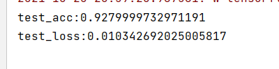
test_loss, test_acc = model.evaluate_generator(test_generator, steps=50)
print('test_acc:' + str(test_acc))
print('test_loss:' + str(test_loss))
小结
我们最终得到了 将近93%精度。
1、卷积神经网络是用于计算机视觉的最佳机器学习模型。即使在非常小的数据集上也可以训练一个卷积神经网络,而且得到的效果不错。
2、小型数据集上主要的问题就是“过拟合”。在处理图像数据时,“数据增强”是一种降低“过拟合”的强大方法。
3、利用“特征提取”,很容易将现有的卷积神经网络复用到新的数据集上。
4、使用“模型微调”提高模型的性能。
14.总结
通过本小结我本人学到了太多太多的东西了;无奈篇幅过于长,但是里面都是干货。我真正意义上实现了一个“猫狗识别”的卷积神经网络的小案例。在后面有一个“卷积神经网络的可视化”,利用当前训练并保存好的模型,可以实现可视化。
15 网盘链接
很早之前自己敲过的代码,在最后分享一下叭,里面有我写过的代码和处理过的小型数据集和一些模型。
链接:https://pan.baidu.com/s/1tp6m-GOi6kP2ZUvJNKqs-A
提取码:djjy


 3964
3964


 被折叠的 条评论
为什么被折叠?
被折叠的 条评论
为什么被折叠?
 到【灌水乐园】发言


