【卷积神经网络】CNN详解以及猫狗识别实例

最新推荐文章于 2024-02-17 16:44:41 发布

clyrjj

最新推荐文章于 2024-02-17 16:44:41 发布

阅读量6.7k

点赞数 7

分类专栏：人工智能与机器学习文章标签：人工智能卷积神经网络

本文链接：https://blog.csdn.net/clyrjj/article/details/118003286

版权

人工智能与机器学习专栏收录该内容

13 篇文章 3 订阅

订阅专栏

一、卷积神经网络（CNN）介绍

卷积神经网络（Convolutional Neural Networks, CNN）是一类包含卷积计算且具有深度结构的前馈神经网络（Feedforward Neural Networks），是深度学习（deep learning）的代表算法之一。
顾名思义，就是将卷积与前馈神经网络结合，所衍生出来的一种深度学习算法。

1.1 整体结构

输入层
用于数据的输入
卷积层
使用卷积核进行特征提取和特征映射
激励层
由于卷积也是一种线性运算，因此需要增加非线性映射
池化层
进行下采样，对特征图稀疏处理，减少数据运算量。
全连接层
通常在CNN的尾部进行重新拟合，减少特征信息的损失

1.2 说明

卷积层（包含有卷积核、卷积层参数、激励函数）：使用卷积核进行特征提取和特征映射。
卷积核
类似于一个前馈神经网络的神经元，组成卷积核的每个元素都对应一个权重系数核一个偏差量，含义可类比视觉皮肤细胞的感受野
卷积层参数
包括卷积核大小、步长、填充，三者共同决定了卷积层输出特征图的尺寸，是卷积神经网络的超参数
激励函数
协助表达复杂的特征，类似于其它深度学习算法

在这里插入图片描述

池化层
最大池化，它只是输出在区域中观察到的最大输入值
均值池化，它只是输出在区域中观察到的平均输入值
两者最大区别在于卷积核的不同（池化是一种特殊的卷积过程）
全连接层

卷积神经网络中的全连接层等价于传统前馈神经网络中的隐含层（每个神经元与上一层的所有神经元相连）全连接层位于卷积神经网络隐含层的最后部分，并只向其它全连接层传递信号。特征图在全连接层中会失去空间拓扑结构，被展开为向量并通过激励函数。全连接层的作用则是对提取的特征进行非线性组合以得到输出，即全连接层本身不被期望具有特征提取能力，而是试图利用现有的高阶特征完成学习目标。

在这里插入图片描述

1.3 特点

局部连接
每个神经元不再和上一层的所有神经元相连，而只和一小部分神经元相连。这样就减少了很多参数。
权值共享
一组连接可以共享同一个权重，而不是每个连接有一个不同的权重，这样又减少了很多参数。
下采样
可以使用Pooling来减少每层的样本数，进一步减少参数数量，同时还可以提升模型的鲁棒性。

1.4 应用领域

在计算机视觉中应用于：图像识别、物体识别、行为认知、姿态估计、神经风格迁移。
也应用于自然语言处理与物理学、遥感科学、大气科学等其他领域。

二、配置实验环境

1、
安装Anaconda

2、
创建虚拟环境
打开cmd

conda create -n tf1 python=3.6

3、
激活环境

activate
conda activate tf1

4、
安装 tensorflow、keras 库
在这里插入图片描述

pip install tensorflow==1.14.0 -i “https://pypi.doubanio.com/simple/”
pip install keras==2.2.5 -i “https://pypi.doubanio.com/simple/”

5、
安装 nb_conda_kernels 包。

conda install nb_conda_kernels

6、
打开 Jupyter Notebook（tf1）环境下的
在这里插入图片描述

三、猫狗识别实例

3.1 准备数据集

在数据分析处理这一块，原数据模型是最值价的了，常用的是kaggle网站的数据集

从Kaggle下载猫狗数据集
百度云链接：https://pan.baidu.com/s/13hw4LK8ihR6-6-8mpjLKDA
密码：dmp4
下载好的原始数据集

3.2 图片分类

代码如下

import os, shutil
# The path to the directory where the original
# dataset was uncompressed
original_dataset_dir = 'D:/python_project/kaggle_Dog&Cat/train'

# The directory where we will
# store our smaller dataset
base_dir = 'D:/python_project/kaggle_Dog&Cat/find_cats_and_dogs'
os.mkdir(base_dir)

# Directories for our training,
# validation and test splits
train_dir = os.path.join(base_dir, 'train')
os.mkdir(train_dir)
validation_dir = os.path.join(base_dir, 'validation')
os.mkdir(validation_dir)
test_dir = os.path.join(base_dir, 'test')
os.mkdir(test_dir)

# Directory with our training cat pictures
train_cats_dir = os.path.join(train_dir, 'cats')
os.mkdir(train_cats_dir)

# Directory with our training dog pictures
train_dogs_dir = os.path.join(train_dir, 'dogs')
os.mkdir(train_dogs_dir)

# Directory with our validation cat pictures
validation_cats_dir = os.path.join(validation_dir, 'cats')
os.mkdir(validation_cats_dir)

# Directory with our validation dog pictures
validation_dogs_dir = os.path.join(validation_dir, 'dogs')
os.mkdir(validation_dogs_dir)

# Directory with our validation cat pictures
test_cats_dir = os.path.join(test_dir, 'cats')
os.mkdir(test_cats_dir)

# Directory with our validation dog pictures
test_dogs_dir = os.path.join(test_dir, 'dogs')
os.mkdir(test_dogs_dir)

# Copy first 1000 cat images to train_cats_dir
fnames = ['cat.{}.jpg'.format(i) for i in range(1000)]
for fname in fnames:
    src = os.path.join(original_dataset_dir, fname)
    dst = os.path.join(train_cats_dir, fname)
    shutil.copyfile(src, dst)

# Copy next 500 cat images to validation_cats_dir
fnames = ['cat.{}.jpg'.format(i) for i in range(1000, 1500)]
for fname in fnames:
    src = os.path.join(original_dataset_dir, fname)
    dst = os.path.join(validation_cats_dir, fname)
    shutil.copyfile(src, dst)
    
# Copy next 500 cat images to test_cats_dir
fnames = ['cat.{}.jpg'.format(i) for i in range(1500, 2000)]
for fname in fnames:
    src = os.path.join(original_dataset_dir, fname)
    dst = os.path.join(test_cats_dir, fname)
    shutil.copyfile(src, dst)
    
# Copy first 1000 dog images to train_dogs_dir
fnames = ['dog.{}.jpg'.format(i) for i in range(1000)]
for fname in fnames:
    src = os.path.join(original_dataset_dir, fname)
    dst = os.path.join(train_dogs_dir, fname)
    shutil.copyfile(src, dst)
    
# Copy next 500 dog images to validation_dogs_dir
fnames = ['dog.{}.jpg'.format(i) for i in range(1000, 1500)]
for fname in fnames:
    src = os.path.join(original_dataset_dir, fname)
    dst = os.path.join(validation_dogs_dir, fname)
    shutil.copyfile(src, dst)
    
# Copy next 500 dog images to test_dogs_dir
fnames = ['dog.{}.jpg'.format(i) for i in range(1500, 2000)]
for fname in fnames:
    src = os.path.join(original_dataset_dir, fname)
    dst = os.path.join(test_dogs_dir, fname)
    shutil.copyfile(src, dst)

统计图片数量

print('total training cat images:', len(os.listdir(train_cats_dir)))
print('total training dog images:', len(os.listdir(train_dogs_dir)))
print('total validation cat images:', len(os.listdir(validation_cats_dir)))
print('total validation dog images:', len(os.listdir(validation_dogs_dir)))
print('total test cat images:', len(os.listdir(test_cats_dir)))
print('total test dog images:', len(os.listdir(test_dogs_dir)))

在这里插入图片描述

分类完毕的文件夹

3.3 网络模型搭建

model.summary()输出模型各层的参数状况

from keras import layers
from keras import models

model = models.Sequential()
model.add(layers.Conv2D(32, (3, 3), activation='relu',
                        input_shape=(150, 150, 3)))
model.add(layers.MaxPooling2D((2, 2)))
model.add(layers.Conv2D(64, (3, 3), activation='relu'))
model.add(layers.MaxPooling2D((2, 2)))
model.add(layers.Conv2D(128, (3, 3), activation='relu'))
model.add(layers.MaxPooling2D((2, 2)))
model.add(layers.Conv2D(128, (3, 3), activation='relu'))
model.add(layers.MaxPooling2D((2, 2)))
model.add(layers.Flatten())
model.add(layers.Dense(512, activation='relu'))
model.add(layers.Dense(1, activation='sigmoid'))
model.summary()

在这里插入图片描述

3.4 训练前准备

配置优化器：
loss：计算损失，这里用的是交叉熵损失
metrics：列表，包含评估模型在训练和测试时的性能的指标

from keras import optimizers

model.compile(loss='binary_crossentropy',
              optimizer=optimizers.RMSprop(lr=1e-4),
              metrics=['acc'])

图片格式转化
所有图片（2000张）重设尺寸大小为 150x150 大小，并使用 ImageDataGenerator 工具将本地图片 .jpg 格式转化成 RGB 像素网格，再转化成浮点张量上传到网络上。

from keras.preprocessing.image import ImageDataGenerator

# 所有图像将按1/255重新缩放
train_datagen = ImageDataGenerator(rescale=1./255)
test_datagen = ImageDataGenerator(rescale=1./255)

train_generator = train_datagen.flow_from_directory(
        # 这是目标目录
        train_dir,
        # 所有图像将调整为150x150
        target_size=(150, 150),
        batch_size=20,
        # 因为我们使用二元交叉熵损失，我们需要二元标签
        class_mode='binary')

validation_generator = test_datagen.flow_from_directory(
        validation_dir,
        target_size=(150, 150),
        batch_size=20,
        class_mode='binary')

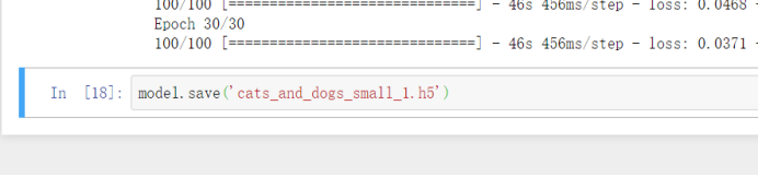
3.5 开始训练

generator()

#模型训练过程
history = model.fit_generator(
      train_generator,
      steps_per_epoch=100,
      epochs=30,
      validation_data=validation_generator,
      validation_steps=50)

在这里插入图片描述

保存模型

#保存训练得到的的模型
model.save('C:\\Res\Cat_And_Dog\\kaggle\\cats_and_dogs_small_1.h5')

在这里插入图片描述

3.6 结果可视化

#对于模型进行评估，查看预测的准确性
import matplotlib.pyplot as plt

acc = history.history['acc']
val_acc = history.history['val_acc']
loss = history.history['loss']
val_loss = history.history['val_loss']

epochs = range(len(acc))

plt.plot(epochs, acc, 'bo', label='Training acc')
plt.plot(epochs, val_acc, 'b', label='Validation acc')
plt.title('Training and validation accuracy')
plt.legend()

plt.figure()

plt.plot(epochs, loss, 'bo', label='Training loss')
plt.plot(epochs, val_loss, 'b', label='Validation loss')
plt.title('Training and validation loss')
plt.legend()

plt.show()

在这里插入图片描述

由可视化结果可知训练的loss是成上升趋势。很明显模型上来就过拟合了，主要原因是数据不够，或者说相对于数据量，模型过复杂。

过拟合：给定一个假设空间 H ，一个假设 h 属于 H ，如果存在其他的假设 h * 属于 H ，使得在训练样例上 h 的错误率比 h * 小，但在整个实例分布上 h * 比 h 的错误率小，那么就说假设 h 过度拟合训练数据。

四、根据基准模型进行调整

为了解决过拟合问题，可以减小模型复杂度，也可以用一系列手段去对冲，比如增加数据（图像增强、人工合成或者多搜集真实数据）、L1/L2正则化、dropout正则化等。这里主要介绍CV中最常用的图像增强。

4.1图形增强方法

在Keras中，可以利用图像生成器很方便地定义一些常见的图像变换。将变换后的图像送入训练之前，可以按变换方法逐个看看变换的效果。

from keras.preprocessing.image import ImageDataGenerator
datagen = ImageDataGenerator(
      rotation_range=40,
      width_shift_range=0.2,
      height_shift_range=0.2,
      shear_range=0.2,
      zoom_range=0.2,
      horizontal_flip=True,
      fill_mode='nearest')

在这里插入图片描述

4.2 查看数据增强后的效果

import matplotlib.pyplot as plt
# This is module with image preprocessing utilities
from keras.preprocessing import image
fnames = [os.path.join(train_cats_dir, fname) for fname in os.listdir(train_cats_dir)]
# We pick one image to "augment"
img_path = fnames[3]
# Read the image and resize it
img = image.load_img(img_path, target_size=(150, 150))
# Convert it to a Numpy array with shape (150, 150, 3)
x = image.img_to_array(img)
# Reshape it to (1, 150, 150, 3)
x = x.reshape((1,) + x.shape)
# The .flow() command below generates batches of randomly transformed images.
# It will loop indefinitely, so we need to `break` the loop at some point!
i = 0
for batch in datagen.flow(x, batch_size=1):
    plt.figure(i)
    imgplot = plt.imshow(image.array_to_img(batch[0]))
    i += 1
    if i % 4 == 0:
        break
plt.show()

在这里插入图片描述

4.3 准备训练并开始训练

图片格式转换

train_datagen = ImageDataGenerator(
    rescale=1./255,
    rotation_range=40,
    width_shift_range=0.2,
    height_shift_range=0.2,
    shear_range=0.2,
    zoom_range=0.2,
    horizontal_flip=True,)
# Note that the validation data should not be augmented!
test_datagen = ImageDataGenerator(rescale=1./255)
train_generator = train_datagen.flow_from_directory(
        # This is the target directory
        train_dir,
        # All images will be resized to 150x150
        target_size=(150, 150),
        batch_size=32,
        # Since we use binary_crossentropy loss, we need binary labels
        class_mode='binary')
validation_generator = test_datagen.flow_from_directory(
        validation_dir,
        target_size=(150, 150),
        batch_size=32,
        class_mode='binary')

开始训练并保存结果

history = model.fit_generator(
      train_generator,
      steps_per_epoch=100,
      epochs=100,
      validation_data=validation_generator,
      validation_steps=50)
model.save('C:\\Res\Cat_And_Dog\\kaggle\\cats_and_dogs_small_2.h5')

在这里插入图片描述

结果可视化

acc = history.history['acc']
val_acc = history.history['val_acc']
loss = history.history['loss']
val_loss = history.history['val_loss']
epochs = range(len(acc))
plt.plot(epochs, acc, 'bo', label='Training acc')
plt.plot(epochs, val_acc, 'b', label='Validation acc')
plt.title('Training and validation accuracy')
plt.legend()
plt.figure()
plt.plot(epochs, loss, 'bo', label='Training loss')
plt.plot(epochs, val_loss, 'b', label='Validation loss')
plt.title('Training and validation loss')
plt.legend()
plt.show()

在这里插入图片描述

五、使用VGG19实现猫狗分类

5.1 初始化一个VGG19网络实例

from keras.applications import VGG19
conv_base = VGG19(weights = 'imagenet',include_top = False,input_shape=(150, 150, 3))
conv_base.summary()

5.2 神经网络接收数据集信息

import os 
import numpy as np
from keras.preprocessing.image import ImageDataGenerator
# 数据集分类后的目录
base_dir = 'E:\\Cat_And_Dog\\kaggle\\cats_and_dogs_small'
train_dir = os.path.join(base_dir, 'train')
validation_dir = os.path.join(base_dir, 'validation')
test_dir = os.path.join(base_dir, 'test')
datagen = ImageDataGenerator(rescale = 1. / 255)
batch_size = 20
def extract_features(directory, sample_count):
    features = np.zeros(shape = (sample_count, 4, 4, 512))
    labels = np.zeros(shape = (sample_count))
    generator = datagen.flow_from_directory(directory, target_size = (150, 150), 
                                            batch_size = batch_size,
                                            class_mode = 'binary')
    i = 0
    for inputs_batch, labels_batch in generator:
        #把图片输入VGG16卷积层，让它把图片信息抽取出来
        features_batch = conv_base.predict(inputs_batch)
        #feature_batch 是 4*4*512结构
        features[i * batch_size : (i + 1)*batch_size] = features_batch
        labels[i * batch_size : (i+1)*batch_size] = labels_batch
        i += 1
        if i * batch_size >= sample_count :
            #for in 在generator上的循环是无止境的，因此我们必须主动break掉
            break
        return features , labels
#extract_features 返回数据格式为(samples, 4, 4, 512)
train_features, train_labels = extract_features(train_dir, 2000)
validation_features, validation_labels = extract_features(validation_dir, 1000)
test_features, test_labels = extract_features(test_dir, 1000)

5.3 训练

将抽取的特征输入到我们自己的神经层中进行分类训练

train_features = np.reshape(train_features, (2000, 4 * 4 * 512))
validation_features = np.reshape(validation_features, (1000, 4 * 4 * 512))
test_features = np.reshape(test_features, (1000, 4 * 4* 512))
from keras import models
from keras import layers
from keras import optimizers
#构造我们自己的网络层对输出数据进行分类
model = models.Sequential()
model.add(layers.Dense(256, activation='relu', input_dim = 4 * 4 * 512))
model.add(layers.Dropout(0.5))
model.add(layers.Dense(1, activation = 'sigmoid'))
model.compile(optimizer=optimizers.RMSprop(lr = 2e-5), loss = 'binary_crossentropy', metrics = ['acc'])
history = model.fit(train_features, train_labels, epochs = 30, batch_size = 20, 
                    validation_data = (validation_features, validation_labels))

在这里插入图片描述

5.4 结果可视化

import matplotlib.pyplot as plt
acc = history.history['acc']
val_acc = history.history['val_acc']
loss = history.history['loss']
val_loss = history.history['val_loss']
epochs = range(1, len(acc) + 1)
plt.plot(epochs, acc, 'bo', label = 'Train_acc')
plt.plot(epochs, val_acc, 'b', label = 'Validation acc')
plt.title('Trainning and validation accuracy')
plt.legend()
plt.figure()
plt.plot(epochs, loss, 'bo', label = 'Training loss')
plt.plot(epochs, val_loss, 'b', label = 'Validation loss')
plt.title('Training and validation loss')
plt.legend()
plt.show()