使用 Python 探索物理实验数据：温度变化曲线绘制与分析

      在物理实验中，数据的可视化和分析对于理解实验结果至关重要。本文将介绍如何使用 Python 和 Matplotlib 库来处理和可视化实验数据，具体包括绘制升温和冷却过程的温度变化曲线，以及计算冷却速率和导热系数。通过这个案例，能够学习到如何有效地应用 Python 工具处理科学数据，并进行初步的数据分析。

数据处理与曲线绘制

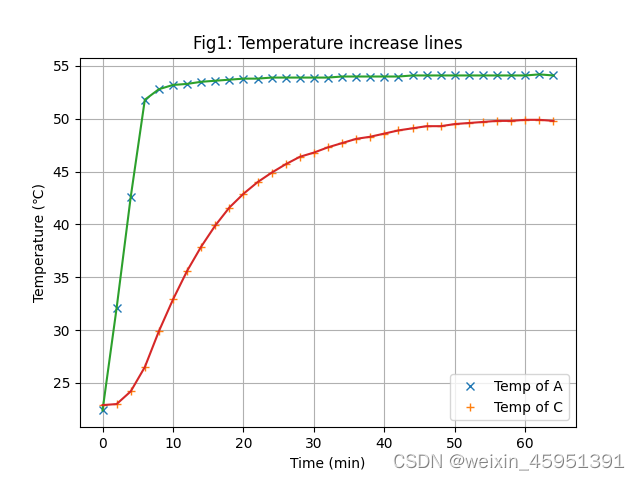
在本实验中，记录了某物体在升温和冷却过程中的温度变化。通过绘制温度变化曲线，可以直观地观察温度随时间的变化趋势。

import numpy as np
import matplotlib.pyplot as plt

# 这里我们导入实验测得的温度数据和时间数据
T_A = np.array([...])  # A盘温度数据
T_C = np.array([...])  # C盘温度数据
time = np.arange(0, 2 * len(T_A), 2)  # 升温过程时间

# 使用 Matplotlib 绘制温度变化曲线
plt.plot(time, T_A, 'x', time, T_C, '+', time, T_A, time, T_C)
plt.legend(['Temp of A', 'Temp of C'])
plt.xlabel('Time (min)')
plt.ylabel('Temperature (℃)')
plt.title('Temperature Increase Lines')
plt.grid()
plt.show()

冷却速率和导热系数的计算

接下来，计算冷却过程中的冷却速率，以及基于实验数据计算待测样品的导热系数。

# 计算冷却速率
k = np.array([...])
print('冷却速率为：{:.3f} ℃/s'.format(k))

# 导热系数计算
m = ...  # 散热盘C质量
C = ...  # 散热盘C比热
# 更多相关物理参数
x = ...
print('导热系数为：{:.3f} W/(m·K)'.format(x))

完整代码

import numpy as np
import matplotlib.pyplot as plt

#%%
# 升温过程的A, C盘温度，单位：℃
T_A = np.array([22.4, 32.1, 42.6, 51.8, 52.8, 53.2, 53.3, 53.5, 53.6, 53.7,
                53.8, 53.8, 53.9, 53.9, 53.9, 53.9, 53.9, 54.0, 54.0, 54.0,
                54.0, 54.0, 54.1, 54.1, 54.1, 54.1, 54.1, 54.1, 54.1, 54.1,
                54.1, 54.2, 54.1])
T_C = np.array([22.9, 23.0, 24.2, 26.5, 29.9, 32.9, 35.6, 37.9, 39.9, 41.6,
                42.9, 44.0, 44.9, 45.7, 46.4, 46.8, 47.3, 47.7, 48.1, 48.3,
                48.6, 48.9, 49.1, 49.3, 49.3, 49.5, 49.6, 49.7, 49.8, 49.8,
                49.9, 49.9, 49.8])
# 升温过程时间，间隔：2min，单位：min
time = np.arange(0, 2*T_A.size, 2)

#%%
# 绘制升温过程A, B盘的温度变化曲线
plt.plot(time, T_A, 'x', time, T_C, '+', time, T_A, time, T_C)
plt.legend(['Temp of A', 'Temp of C'])
plt.xlabel('Time (min)')
plt.ylabel('Temperature (℃)')
plt.title('Fig1: Temperature increase lines')
plt.grid()
plt.savefig('Fig1_Temp_inrease.png')
plt.show()

#%%
# 冷却过程C盘温度，单位：℃
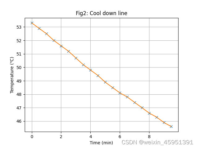
T_C_2 = np.array([53.3, 52.9, 52.5, 52.0, 51.6, 51.2, 50.7, 50.2, 49.8, 49.4,
                  48.9, 48.5, 48.1, 47.8, 47.4, 47.0, 46.6, 46.3, 45.9, 45.6])
T_10 = T_C_2[-11:-1]
# 冷却过程时间，间隔：30s 单位：min
time_2 = np.arange(0, 0.5*T_C_2.size, 0.5)
time_2_s = time_2 * 60  # 以秒为单位的时间，后面计算不确定度时会用到

#%%
# 绘制冷却过程曲线
plt.plot(time_2, T_C_2, 'x', time_2, T_C_2)
plt.xlabel('Time (min)')
plt.ylabel('Temperature (℃)')
plt.title('Fig2: Cool down line')
plt.grid()
plt.savefig('Fig2_cool_down.png')
plt.show()

#%%
# 取T2附近10个点用逐差法计算冷却速率：k = dT/dt，单位：℃/s
k =  np.array([T_10[i]-T_10[i+5] for i in range(5)]).sum() / (25 * 30)
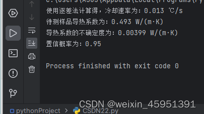
print('使用逐差法计算得，冷却速率为：{:.3f} ℃/s'.format(k))

#%%
# 计算待测样品的导热系数
# 散热盘C质量 m，单位：kg
m = 0.68
# 散热盘C比热 C，单位：J/(kg·℃)
C = 394
# 散热盘C密度 d，单位：kg/m^(3)
d = 8.9 * 1000
# 散热盘C半径 Rc，单位：m
Rc = 99.908 * 0.001 / 2
# 散热盘C厚度 hc，单位：m
hc = 8.832 * 0.001
# 发热盘B半径 Rb，单位：m
Rb = 99.976 * 0.001 / 2
# 发热盘B厚度 hb，单位：m
hb = 8.492 * 0.001
# A盘稳态温度T1，单位：℃
T1 = 54.1
# C盘稳态温度T2，单位：℃
T2 = 49.82

# 计算导热系数x, 单位：W/(m·K)
x = m * C * k * (Rc + 2 * hc) * hb / ((2 * Rc + 2 * hc) * (T1 - T2) * np.pi * Rb ** 2)
print('待测样品导热系数为：{:.3f} W/(m·K)'.format(x))

#%%
# 计算间接测量量热导系数x的不确定度 Ux，讲义上提到，该实验仪器的温度分辨率为：0.1℃，计时分辨率为：0.1s
def ua(x):
    # 计算A类不确定度
    x_array = np.array(x)
    return np.sqrt(x_array.var()/(x_array.size-1))

def U(ua, delta):
    # 计算直接测量量，需传入A类不确定度，和仪器误差
    # 这里，置信概率p取0.95，查表得
    tp = 2.26
    kp = 1.96
    return np.sqrt((tp*ua)**2+(kp*delta/np.sqrt(3))**2)

# 最后计算间接测量量热导系数x的不确定度 Ux
Ux = k * np.sqrt((U(ua(T_10), 0.1)/T_10.mean())**2+(U(ua(time_2_s), 0.1)/time_2_s.mean())**2)
print('导热系数的不确定度为：{:.5f} W/(m·K)'.format(Ux))
print('置信概率为：0.95')

运行结果