◇【论文_20150909v1_20190705v6】Deep DPG (DDPG) 〔Google Deepmind〕【高维连续动作空间 + off-policy】

https://arxiv.org/abs/1509.02971

可参考 Code 实现

Continuous control with deep reinforcement learning

摘要

We adapt the ideas underlying the success of Deep Q-Learning to the continuous action domain. 【研究范围】
我们将 Deep Q-Learning 成功的基础思想应用于连续动作领域。 〔 DQN 用到 连续动作环境 〕
We present an actor-critic, model-free algorithm based on the deterministic policy gradient that can operate over continuous action spaces. 【我们提出了一种… 的…(类别)算法，该算法可以…】
我们提出了一种基于确定性策略梯度的 actor-critic，无模型算法，该算法可以在连续的动作空间上运行。
Using the same learning algorithm, network architecture and hyper-parameters, our algorithm robustly solves more than 20 simulated physics tasks, including classic problems such as cartpole swing-up, dexterous manipulation, legged locomotion and car driving. 【解决了哪些任务】
使用相同的学习算法、网络架构和超参数，我们的算法鲁棒地解决了 20 多个模拟物理任务，包括经典问题，如车杆摆动、灵巧操作、腿部运动和汽车驾驶。
Our algorithm is able to find policies whose performance is competitive with those found by a planning algorithm with full access to the dynamics of the domain and its derivatives. 【优势】
我们的算法能够找到那些性能与 完全访问域及其衍生 动态的规划算法所发现的策略 具有竞争力的策略。
We further demonstrate that for many of the tasks the algorithm can learn policies “end-to-end”: directly from raw pixel inputs. 【像素输入 ——> 策略】
我们进一步证明，对于许多任务，算法可以“端到端”学习策略：直接从原始像素输入。

1 引言

One of the primary goals of the field of artificial intelligence is to solve complex tasks from unprocessed, high-dimensional, sensory input. 【本工作大目标】
人工智能领域的主要目标之一是从未处理的、高维的感官输入中解决复杂的任务。
Recently, significant progress has been made by combining advances in deep learning for sensory processing (Krizhevsky et al., 2012) with reinforcement learning, resulting in the “Deep Q Network” (DQN) algorithm (Mnih et al., 2015) that is capable of human level performance on many Atari video games using unprocessed pixels for input. 【最近的里程碑式进展】
最近，通过将用于感官处理的深度学习（Krizhevsky et al., 2012）与强化学习的进展相结合，取得了重大进展，从而产生了 “Deep Q Network” (DQN) 算法（Mnih et al., 2015），该算法能够在使用未处理像素作为输入的许多 Atari 视频游戏上达到人类水平。
To do so, deep neural network function approximators were used to estimate the action-value function.
为此，使用深度神经网络函数近似器来估计动作价值函数。

However, while DQN solves problems with high-dimensional observation spaces, it can only handle discrete and low-dimensional action spaces. 【DQN 适用的场景】
然而，DQN 在解决高维观测空间问题的同时，只能处理离散的、低维的动作空间。 〔 DQN 适用于 高维观测空间 + 离散低维动作空间〕
Many tasks of interest, most notably physical control tasks, have continuous (real valued) and high dimensional action spaces. 【小目标： 拟考虑的目标场景】
许多有趣的任务，尤其是物理控制任务，具有连续的（实数的）和高维的动作空间。
DQN cannot be straightforwardly applied to continuous domains since it relies on a finding the action that maximizes the action-value function, which in the continuous valued case requires an iterative optimization process at every step. 【DQN 无法直接用于目标场景的原因】
DQN 不能直接应用于连续域，因为它依赖于找到最大化动作价值函数的动作，而在连续值的情况下，这需要在每一步进行迭代优化过程。

↓ 【DQN 应用于连续域的当前改进方案 存在的不足】

An obvious approach to adapting deep reinforcement learning methods such as DQN to continuous domains is to to simply discretize the action space.
将深度强化学习方法（如 DQN）应用于连续域的一个明显方法是简单地离散动作空间。
However, this has many limitations, most notably the curse of dimensionality: the number of actions increases exponentially with the number of degrees of freedom.
然而，这有许多限制，最明显的是维度的魔咒：动作的数量随着自由度的增加呈指数增长。
For example, a 7 degree of freedom system (as in the human arm) with the coarsest discretization a i ∈ { − k , 0 , k } a_i \in\{-k, 0, k\} ai​∈{−k,0,k} for each joint leads to an action space with dimensionality: $3^7=2187$.
例如，一个自由度为 7 的系统（如在人类手臂中），每个关节的最粗离散化 a i ∈ { − k , 0 , k } a_i \in\{-k, 0, k\} ai​∈{−k,0,k} 导致一个维度为 $3^7=2187$ 的动作空间。
The situation is even worse for tasks that require fine control of actions as they require a correspondingly finer grained discretization, leading to an explosion of the number of discrete actions.
对于需要精细控制动作的任务，情况甚至更糟，因为它们需要相应的更细粒度的离散化，从而导致离散动作数量的激增。
Such large action spaces are difficult to explore efficiently, and thus successfully training DQN-like networks in this context is likely intractable.
如此大的动作空间很难有效地探索，因此在这种情况下成功训练类似 DQN 的网络可能是棘手的。
Additionally, naive discretization of action spaces needlessly throws away information about the structure of the action domain, which may be essential for solving many problems.
此外，简单的动作空间离散化不必要地丢弃了关于动作域结构的信息，而这些信息对于解决许多问题可能是必不可少的。

↓ 【本文工作 + 受谁启发 (+ 这些方法的不足)】

In this work we present a model-free, off-policy actor-critic algorithm using deep function approximators that can learn policies in high-dimensional, continuous action spaces.
在这项工作中，我们提出了一种使用深度函数近似器的无模型、异策略off-policy 行为者-评论员actor-critic 算法，该算法可以在高维连续动作空间中学习策略。
Our work is based on the deterministic policy gradient (DPG) algorithm (Silver et al., 2014) (itself similar to NFQCA (Hafner & Riedmiller, 2011), and similar ideas can be found in (Prokhorov et al., 1997)).
我们的工作基于确定性策略梯度（DPG）算法（Silver et al., 2014）(本身类似于 NFQCA （Hafner & Riedmiller, 2011)，在（Prokhorov et al., 1997）中可以找到类似的想法）。
However, as we show below, a naive application of this actor-critic method with neural function approximators is unstable for challenging problems.
然而，正如我们在下面所展示的，这种带有神经函数近似器的 actor-critic 方法的幼稚应用对于具有挑战性的问题是不稳定的。

↓ 【关键 idea + 相关要点】

Here we combine the actor-critic approach with insights from the recent success of Deep Q Network (DQN) (Mnih et al., 2013; 2015).
在这里，我们将 actor-critic 方法与深度 Q 网络（DQN） (Mnih 等人，2013；2015) 最近成功的见解结合起来。
Prior to DQN, it was generally believed that learning value functions using large, non-linear function approximators was difficult and unstable.
在 DQN 出现之前，人们普遍认为使用大型非线性函数近似器学习价值函数是困难且不稳定的。
DQN is able to learn value functions using such function approximators in a stable and robust way due to two innovations: 1. the network is trained off-policy with samples from a replay buffer to minimize correlations between samples; 2. the network is trained with a target Q network to give consistent targets during temporal difference backups.
DQN 能够使用这种函数近似器以稳定和鲁棒的方式学习价值函数 是由于两个创新：1. 该网络使用来自重放缓冲区replay buffer 的样本以 异策略off-policy 的方式进行训练，以最小化样本之间的相关性；2. 利用目标 Q 网络对网络进行训练，使网络在时序差分备份过程中得到一致的目标。
In this work we make use of the same ideas, along with batch normalization (Ioffe & Szegedy, 2015), a recent advance in deep learning.
在这项工作中，我们使用了相同的思想，以及批标准化batch normalization（ioffe&szegedy, 2015），这是深度学习的最新进展。

↓ 【评估的任务】

In order to evaluate our method we constructed a variety of challenging physical control problems that involve complex multi-joint movements, unstable and rich contact dynamics, and gait behavior.
Among these are classic problems such as the cartpole swing-up problem, as well as many new domains.
为了评估我们的方法，我们构建了各种具有挑战性的物理控制问题，包括复杂的多关节运动，不稳定且丰富的接触动力学以及步态行为。
在这些问题中有经典的问题，如车杆 swing-up 问题，以及许多新的领域。
A long-standing challenge of robotic control is to learn an action policy directly from raw sensory input such as video.
机器人控制的一个长期挑战是直接从原始感官输入（如视频）中学习动作策略。
Accordingly, we place a fixed viewpoint camera in the simulator and attempted all tasks using both low-dimensional observations (e.g. joint angles) and directly from pixels.
因此，我们在模拟器中放置了一个固定视点摄像机，并尝试使用低维观测（例如关节角度）和直接从像素进行所有任务。

↓ 【Deep DPG (DDPG) 优势】

Our model-free approach which we call Deep DPG (DDPG) can learn competitive policies for all of our tasks using low-dimensional observations (e.g. cartesian coordinates or joint angles) using the same hyper-parameters and network structure.
我们的无模型方法，我们称之为 Deep DPG (DDPG)，可以使用相同的超参数和网络结构，使用低维观测（例如笛卡尔坐标或关节角度）学习所有任务的有竞争力的策略。
In many cases, we are also able to learn good policies directly from pixels, again keeping hyperparameters and network structure constant .
在许多情况下，我们也能够直接从像素中学习好的策略，再次保持超参数和网络结构不变。

• 脚注 1： You can view a movie of some of the learned policies at https://goo.gl/J4PIAz
  习得的策略的视频

A key feature of the approach is its simplicity: it requires only a straightforward actor-critic architecture and learning algorithm with very few “moving parts”, making it easy to implement and scale to more difficult problems and larger networks.
该方法的一个关键特点是它的简单性：它只需要一个直接的 actor-critic 架构和学习算法，只有很少的“活动部分”，这使得它很容易实现和扩展到更困难的问题和更大的网络。
For the physical control problems we compare our results to a baseline computed by a planner (Tassa et al., 2012) that has full access to the underlying simulated dynamics and its derivatives (see supplementary information).
对于物理控制问题，我们将结果与规划器（Tassa et al., 2012）计算的基线进行比较，该规划器可以完全访问潜在的模拟动力学及其衍生物（见补充信息）。
Interestingly, DDPG can sometimes find policies that exceed the performance of the planner, in some cases even when learning from pixels (the planner always plans over the underlying low-dimensional state space).
有趣的是，DDPG 有时可以找到超出规划器性能的策略，在某些情况下甚至是在从像素学习时（规划器总是在底层低维状态空间上进行规划）。

2 背景

我们考虑一个标准的强化学习设置，由一个代理agent 与 离散时间步的环境 $E$ 交互组成。
在每个时间步 $t$ 上，agent 接收到一个观察 $x_t$，执行一个动作 $a_t$，并收到一个标量奖励 $r_t$。
在这里考虑的所有环境中，动作是实数的 $a_t\in {\mathbb{R}}^N$。
一般情况下，环境可部分观测，使 整个观测历史，动作对 可能需要用来描述状态 $s_t=(x_1,a_1,\cdots ，a_{t-1},x_t)$ 。
这里，我们假设环境是完全可观测到的，所以 $s_t=x_t$。

agent 的行为由策略 $\pi$ 定义，策略 $\pi$ 将状态映射到动作上的概率分布 $\pi :\mathcal{S}\to \mathcal{P}(\mathcal{A})$ 。
环境 $E$ 也可能是随机的。
我们将其建模为具有状态空间为 $\mathcal{S}$ 、动作空间 $\mathcal{A}={\mathbb{R}}^N$、初始状态分布为 $p(s_1)$、转换动态为 $p(s_{t+1}|s_t,a_t)$ 和奖励函数为 $r(s_t,a_t)$ 的马尔可夫决策过程。

一种状态的回报return 定义为折扣未来奖励和 $R_t=\sum _{i=t}^T{\gamma }^{(i-t)}r(s_i,a_i)$，其中折扣因子 $\gamma \in [0,1]$。
注意，回报取决于所选择的动作，因此取决于策略 $\pi$，并且可能是随机的。
强化学习的目标是学习一种策略，使初始分布 $J={\mathbb{E}}_{r_i,s_i\sim E,a_i\sim \pi }[R_1]$ 的回报期望最大化。
我们用 ${\rho }^{\pi }$ 表示一个策略 $\pi$ 的折扣状态访问分布。

动作价值函数被用于许多强化学习算法中。
它描述了在状态 $s_t$ 下执行动作 $a_t$ 且随后遵循策略 $\pi$ 的回报期望：
  ~  
$Q^{\pi }(s_t,a_t)={\mathbb{E}}_{r_{i\ge t},s_{i>t}\sim E,a_{i>t}\sim \pi }[R_t|s_t,a_t](1)$

Many approaches in reinforcement learning make use of the recursive relationship known as the Bellman equation:
强化学习中的许多方法都利用了被称为 Bellman 公式的递归关系：
  ~  
$Q^{\pi }(s_t,a_t)={\mathbb{E}}_{r_t,s_{t+1}\sim E}[r(s_t,a_t)+\gamma {\mathbb{E}}_{a_{t+1}\sim \pi }[Q^{\pi }(s_{t+1},a_{t+1})]](2)$
  ~  
如果目标策略是确定性的，我们可以将其描述为函数 $\mu :\mathcal{S}\leftarrow \mathcal{A}$，并避免内部期望：
  ~  
$Q^{\mu }(s_t,a_t)={\mathbb{E}}_{r_t,s_{t+1}\sim E}[r(s_t,a_t)+\gamma Q^{\mu }(s_{t+1},\mu (s_{t+1}))](3)$
  ~  
期望只取决于环境。
这意味着可以以 异策略off-policy 的方式学习 $Q^{\mu }$， 使用由不同的随机行为策略 $\beta$ 产生的转换来学习。

Q-learning （Watkins & Dayan, 1992）是一种常用的 off-policy 算法，它使用贪心策略 $\mu (s)=\arg {\max }_{a}Q(s,a)$。
我们考虑参数化为 ${\theta }^Q$ 的函数近似器，我们通过最小化损失来优化它：
  ~  
$L({\theta }^Q)={\mathbb{E}}_{s_t\sim {\rho }^{\beta },a\sim \beta ,r_t\sim E}\left[\right(Q(s_t,a_t|{\theta }^Q)-y_t{)}^2](4)$
  ~  
其中
  ~  
$y_t=r(s_t,a_t)+\gamma Q(s_{t+1},\mu (s_{t+1})|{\theta }^Q)(5)$
  ~  
虽然 $y_t$ 也依赖于 ${\theta }^Q$，但这通常被忽略。

The use of large, non-linear function approximators for learning value or action-value functions has often been avoided in the past since theoretical performance guarantees are impossible, and practically learning tends to be unstable.
在过去，由于理论上的性能保证是不可能的，而且实际的学习往往是不稳定的，因此经常避免使用大型的非线性函数近似器来学习价值或动作价值函数。
Recently, (Mnih et al., 2013; 2015) adapted the Q-learning algorithm in order to make effective use of large neural networks as function approximators.
最近，(Mnih et al., 2013；2015) 采用 Q-learning 算法，以便有效地利用大型神经网络作为函数近似器。
Their algorithm was able to learn to play Atari games from pixels.
他们的算法能够通过像素来学习玩 Atari 游戏。
In order to scale Q-learning they introduced two major changes: the use of a replay buffer, and a separate target network for calculating $y_t$.
为了扩展 Q-learning，他们引入了两个主要的变化：使用 replay buffer，以及一个单独的目标网络来计算 $y_t$。
We employ these in the context of DDPG and explain their implementation in the next section.
我们将在 DDPG 中使用它们，并在下一节中解释它们的实现。

3 算法

It is not possible to straightforwardly apply Q-learning to continuous action spaces, because in continuous spaces finding the greedy policy requires an optimization of $a_t$ at every timestep; this optimization is too slow to be practical with large, unconstrained function approximators and nontrivial action spaces.
不可能直接将 Q-learning 应用于连续动作空间，因为在连续空间中，寻找贪心策略需要在每个时间步上对 $a_t$ 进行优化；这种优化速度太慢，对于大型、无约束的函数近似器和非平凡的动作空间来说是不切实际的。
Instead, here we used an actor-critic approach based on the DPG algorithm (Silver et al., 2014).
取而代之的是，这里我们使用了基于 DPG 算法的 actor-critic 方法（Silver et al., 2014）。

DPG 算法维护一个参数化的 actor 函数 $\mu (s|{\theta }^{\mu })$，它通过确定地将状态映射到特定的动作来指定当前策略。
critic $Q(s,a)$ 是用贝尔曼公式学习的，就像 Q-learning 一样。
通过将链式法则应用于关于 actor 参数的初始分布 $J$ 的回报期望，actor 被更新：
  ~  
$\begin{array}{rl}{\nabla }_{{\theta }^{\mu }}J& \approx {\mathbb{E}}_{s_t\sim {\rho }^{\beta }}[{\nabla }_{{\theta }^{\mu }}Q(s,a|{\theta }^Q){|}_{s=s_t,a=\mu (s_t|{\theta }^{\mu })}]\\ & ={\mathbb{E}}_{s_t\sim {\rho }^{\beta }}[{\nabla }_{a}Q(s,a|{\theta }^Q){|}_{s=s_t,a=\mu (s_t)}{\nabla }_{{\theta }^{\mu }}\mu (s_t|{\theta }^{\mu }){|}_{s=s_t}]\end{array}(6)$

• 〔 上标 标记这是不同网络的权重，神经网络的权重一般用 $\theta$ 表示，Q 网络的权重为 ${\theta }^Q$，策略 $\mu$ 网络的 权重为 ${\theta }^{\mu }$ 〕

  ~  
Silver et al.（2014）证明了这就是策略梯度，即策略性能的梯度。

• 脚注 2：In practice, as in commonly done in policy gradient implementations, we ignored the discount in the state-visitation distribution ${\rho }^{\beta }$.
  在实践中，正如通常在策略梯度实现中所做的那样，我们忽略状态访问分布 ${\rho }^{\beta }$ 中的折扣。

As with Q learning, introducing non-linear function approximators means that convergence is no longer guaranteed.
与 Q-learning 一样，引入非线性函数近似器意味着收敛性不再得到保证。
However, such approximators appear essential in order to learn and generalize on large state spaces.
然而，为了在大的状态空间上学习和泛化，这样的近似器是必不可少的。
NFQCA (Hafner & Riedmiller, 2011), which uses the same update rules as DPG but with neural network function approximators, uses batch learning for stability, which is intractable for large networks.
NFQCA （Hafner & Riedmiller, 2011）使用与 DPG 相同的更新规则，但使用神经网络函数近似器，使用批量学习来保持稳定性，这对于大型网络来说是难以解决的。
A minibatch version of NFQCA which does not reset the policy at each update, as would be required to scale to large networks, is equivalent to the original DPG, which we compare to here.
小批处理版本的 NFQCA 不会在每次更新时重置策略（这是扩展到大型网络所必需的），相当于我们在这里比较的原始 DPG。 〔 目标网络 〕
Our contribution here is to provide modifications to DPG, inspired by the success of DQN, which allow it to use neural network function approximators to learn in large state and action spaces online.
我们的贡献是在 DQN 成功的启发下对 DPG 进行修改，使其能够使用神经网络函数近似器在线学习大状态和动作空间。
We refer to our algorithm as Deep DPG (DDPG, Algorithm 1).
我们将我们的算法称为 Deep DPG（DDPG，算法 1）。

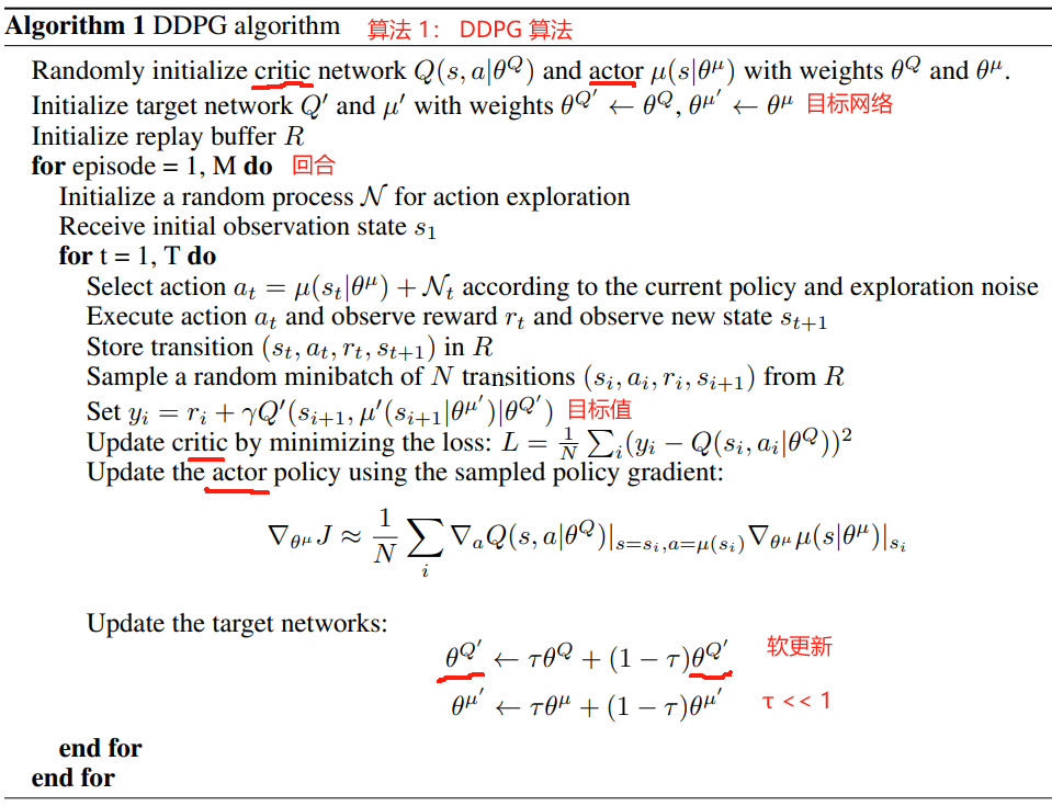
算法 1： DDPG 算法
随机初始化 critic 网络 $Q(s,a|{\theta }^Q)$ 和 actor 网络 $\mu (s|{\theta }^{\mu })$ 的权重 ${\theta }^Q$ 和 ${\theta }^{\mu }$
初始化目标网络 $Q^{\prime }$ 和 ${\mu }^{\prime }$： ${\theta }^{Q^{\prime }}\leftarrow {\theta }^Q$， ${\theta }^{{\mu }^{\prime }}\leftarrow {\theta }^{\mu }$
初始化回放缓冲区replay buffer $R$
$\mathbf{for}$ episode $=1,M\mathbf{do}$ 〔 回合 〕
        ~~~~~~~        初始化随机过程 $\mathcal{N}$ 用于动作探索
        ~~~~~~~        得到初始观测状态 $s_1$
$\mathbf{for}t=1,T\mathbf{do}$ 〔 时间步 〕
               ~~~~~~~~~~~~~~                根据当前策略 和 探索噪声 选择动作 $a_t=\mu (s_t|{\theta }^{\mu })+{\mathcal{N}}_t$
               ~~~~~~~~~~~~~~                执行动作 $a_t$，观测奖励 $r_t$ 和 新状态 $s_{t+1}$
               ~~~~~~~~~~~~~~                存储转换 $(s_t,a_t,r_t,s_{t+1})$ 到 $R$ 中
               ~~~~~~~~~~~~~~                从 $R$ 中随机抽取大小为 $N$ 的小批转换 $(s_i,a_i,r_i,s_{i+1})$
               ~~~~~~~~~~~~~~                令 $y_i=r_i+\gamma Q^{\prime }(s_{i+1},{\mu }^{\prime }(s_{i+1}|{\theta }^{{\mu }^{\prime }})|{\theta }^{Q^{\prime }})$
               ~~~~~~~~~~~~~~                通过最小化损失更新 critic： $L=\frac{1}{N}\sum _i(y_i-Q(s_i,a_i|{\theta }^Q){)}^2$
               ~~~~~~~~~~~~~~                使用采样的策略梯度更新 actor 策略：
${\nabla }_{{\theta }^{\mu }}J\approx \frac{1}{N}\sum _i{\nabla }_{a}Q(s,a|{\theta }^Q){|}_{s=s_i,a=\mu (s_i)}{\nabla }_{{\theta }^{\mu }}\mu (s|{\theta }^{\mu }){|}_{s_i}$
               ~~~~~~~~~~~~~~                更新目标网络： 〔 $\tau \ll 1$ 〕
${\theta }^{Q^{\prime }}\leftarrow \tau {\theta }^Q+(1-\tau ){\theta }^{Q^{\prime }}$
${\theta }^{{\mu }^{\prime }}\leftarrow \tau {\theta }^{\mu }+(1-\tau ){\theta }^{{\mu }^{\prime }}$
$\mathbf{end}\mathbf{for}$
$\mathbf{end}\mathbf{for}$

↓ 【问题 1：优化算法要求样本 独立同分布问题】

One challenge when using neural networks for reinforcement learning is that most optimization algorithms assume that the samples are independently and identically distributed.
使用神经网络进行强化学习的一个挑战是，大多数优化算法都假设样本是独立同分布的。
Obviously, when the samples are generated from exploring sequentially in an environment this assumption no longer holds.
显然，当样本是通过在环境中循序探索而生成时，这个假设就不再成立了。
Additionally, to make efficient use of hardware optimizations, it is essential to learn in minibatches, rather than online.
此外，为了有效地利用硬件优化，有必要进行小批量学习，而不是在线学习。

↓ 【问题 1 的解决方案： 经验回放】

As in DQN, we used a replay buffer to address these issues.
The replay buffer is a finite sized cache $\mathcal{R}$.
在 DQN 中，我们使用了一个重放缓冲区replay buffer 来解决这些问题。
replay buffer 是一个有限大小的缓存 $\mathcal{R}$。
Transitions were sampled from the environment according to the exploration policy and the tuple $(s_t,a_t,r_t,s_{t+1})$ was stored in the replay buffer.
根据探索策略从环境中采样转换，元组 $(s_t,a_t,r_t,s_{t+1})$ 存储在 replay buffer 中。
When the replay buffer was full the oldest samples were discarded.
当 回放缓冲区满时，旧的样本被丢弃。
At each timestep the actor and critic are updated by sampling a minibatch uniformly from the buffer.
在每个时间步，actor 和 critic 通过从缓冲区中均匀采样一个小批来更新。
Because DDPG is an off-policy algorithm, the replay buffer can be large, allowing the algorithm to benefit from learning across a set of uncorrelated transitions.
由于 DDPG 是一种 off-policy 算法，因此重放缓冲区可以很大，从而允许算法从跨一组不相关转换的学习中获益。

↓ 【问题 2：神经网络直接估计 Q 的值 不稳定。
问题 2 的解决方案：软目标更新 】

用神经网络直接实现 Q-learning（式 4）在许多环境中被证明是不稳定的。
由于正在更新的网络 $Q(s,a|{\theta }^Q)$ 也用于计算目标值（式 5），因此 Q 更新容易出现发散。
我们的解决方案类似于（Mnih et al., 2013）中使用的目标网络，但针对 actor-critic 进行了修改，并使用“软”目标更新，而不是直接复制权重。
我们创建了 actor 和 critic 网络的副本，分别为 $Q^{\prime }(s,a|{\theta }^{Q^{\prime }})$ 和 ${\mu }^{\prime }(s|{\theta }^{{\mu }^{\prime }})$，用于计算目标值。
然后通过让这些目标网络缓慢跟踪习得的网络 〔 $\theta$ 〕 来更新这些目标网络的权重 〔 ${\theta }^{\prime }$ 〕： ${\theta }^{\prime }\leftarrow \tau \theta +(1-\tau ){\theta }^{\prime }$，其中 $\tau \ll 1$。

• 〔 目标网络 缓慢跟随 在线网络〕

这意味着目标值被限制为缓慢变化，大大提高了学习的稳定性。
这个简单的改变使相对不稳定的学习动作价值函数的问题更接近于监督学习的情况，这个问题存在鲁棒的解决方案。
我们发现目标 ${\mu }^{\prime }$ 和 $Q^{\prime }$ 都需要有稳定的目标 $y_i$，以便持续训练 critic 而不发散。
这可能会减慢学习速度，因为目标网络会延迟值估计的传播。
然而，在实践中，我们发现学习的稳定性大大超过了这一点。

↓ 【问题 3：观测的不同部分的单位不一样】

When learning from low dimensional feature vector observations, the different components of the observation may have different physical units (for example, positions versus velocities) and the ranges may vary across environments.
当从低维特征向量观测中学习时，观测的不同组成部分可能具有不同的物理单位（例如，位置与速度），并且范围可能因环境而异。
This can make it difficult for the network to learn effectively and may make it difficult to find hyper-parameters which generalise across environments with different scales of state values.
这可能会使网络难以有效地学习，并可能使其难以找到具有不同状态价值尺度的环境中的超参数。

↓ 【问题 3 的解决方案：批规范化batch normalization】

One approach to this problem is to manually scale the features so they are in similar ranges across environments and units.
解决这个问题的一种方法是手动缩放特征，使它们在不同的环境和单位中处于相似的范围。
We address this issue by adapting a recent technique from deep learning called batch normalization (Ioffe & Szegedy, 2015).
我们通过采用一种最新的深度学习技术来解决这个问题，这种技术被称为批规范化batch normalization（ioffe&szegedy, 2015）。
This technique normalizes each dimension across the samples in a minibatch to have unit mean and variance.
该技术将小批量样本中的每个维度标准化，使其具有单位均值和方差。
In addition, it maintains a running average of the mean and variance to use for normalization during testing (in our case, during exploration or evaluation).
此外，它维护平均值和方差的运行平均值，以便在测试期间（在我们的例子中，在探索或评估期间）用于规范化。
In deep networks, it is used to minimize covariance shift during training, by ensuring that each layer receives whitened input.
在深度网络中，通过确保每一层接收到白化的输入来最小化训练过程中的协方差偏移。
In the low-dimensional case, we used batch normalization on the state input and all layers of the μ network and all layers of the Q network prior to the action input (details of the networks are given in the supplementary material).
在低维情况下，我们在动作输入之前对状态输入、$\mu$ 网络的所有层和 $Q$ 网络的所有层使用 batch normalization（网络的详细信息在补充材料中给出）。
With batch normalization, we were able to learn effectively across many different tasks with differing types of units, without needing to manually ensure the units were within a set range.
通过 batch normalization，我们能够有效地学习具有不同类型单元的许多不同任务，而无需手动确保单元在设定范围内。

↓ 【问题 4：探索
问题 4 的解决方案：探索策略 = actor 策略 + 噪声】

A major challenge of learning in continuous action spaces is exploration.
在连续动作空间中学习的一个主要挑战是探索。
An advantage of off-policies algorithms such as DDPG is that we can treat the problem of exploration independently from the learning algorithm.
像 DDPG 这样的异策略算法的一个优点是，我们可以独立于学习算法来处理探索问题。
我们通过将从噪声过程 $\mathcal{N}$ 中采样的噪声添加到我们的 actor 策略中构建了一个探索策略 ${\mu }^{\prime }$
  ~  
${\mu }^{\prime }(s_t)=\mu (s_t|{\theta }_t^{\mu })+\mathcal{N}(7)$
  ~  
$\mathcal{N}$ 可以根据环境选择。
As detailed in the supplementary materials we used an Ornstein-Uhlenbeck process (Uhlenbeck & Ornstein, 1930) to generate temporally correlated exploration for exploration efficiency in physical control problems with inertia (similar use of autocorrelated noise was introduced in (Wawrzyński, 2015)).
正如补充材料中详细介绍的那样，我们使用了 Ornstein-Uhlenbeck 过程（Uhlenbeck & Ornstein, 1930）来生成具有惯性的物理控制问题中的探索效率的时序相关探索（在（Wawrzyński, 2015）中引入了类似的自相关噪声的使用）。

4 结果

We constructed simulated physical environments of varying levels of difficulty to test our algorithm.
我们构建了不同难度的模拟物理环境来测试我们的算法。
This included classic reinforcement learning environments such as cartpole, as well as difficult, high dimensional tasks such as gripper, tasks involving contacts such as puck striking (canada) and locomotion tasks such as cheetah (Wawrzyński, 2009).
这包括经典的强化学习环境，如 cartpole ，以及困难的高维任务，如抓手gripper，涉及接触的任务，如 击打冰球puck striking （加拿大）和运动任务，如 cheetah（Wawrzyński, 2009）。
In all domains but cheetah the actions were torques applied to the actuated joints.
These environments were simulated using MuJoCo (Todorov et al., 2012).
在除 cheetah 外的所有领域中，动作都是施加到驱动关节上的扭矩。
使用 MuJoCo 模拟这些环境（Todorov 等，2012）。
Figure 1 shows renderings of some of the environments used in the task (the supplementary contains details of the environments and you can view some of the learned policies at https://goo.gl/J4PIAz).
图 1 显示了任务中使用的一些环境的效果图（补充部分包含环境的详细信息，https://goo.gl/J4PIAz 可以查看学到的一些策略）

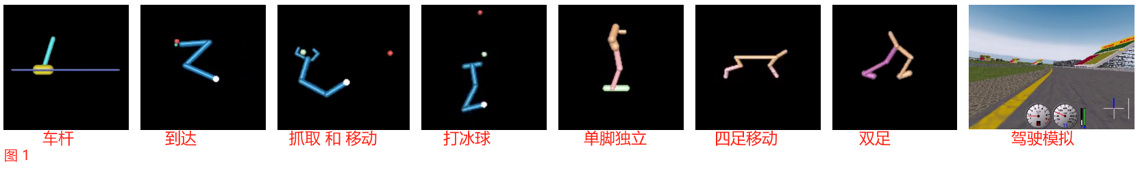
Figure 1: Example screenshots of a sample of environments we attempt to solve with DDPG.
图 1： 我们试图用 DDPG 解决的环境示例截图。
In order from the left: the cartpole swing-up task, a reaching task, a gasp and move task, a puck-hitting task, a monoped balancing task, two locomotion tasks and Torcs (driving simulator).
从左到右依次是：cartpole swing-up 任务，reaching 任务，gasp and move 任务，打冰球任务，单平衡任务，两个运动任务和 Torcs（驾驶模拟器）。
We tackle all tasks using both low-dimensional feature vector and high-dimensional pixel inputs.
我们使用低维特征向量和高维像素输入来处理所有任务。
Detailed descriptions of the environments are provided in the supplementary.
环境的详细描述载于补充文件。
Movies of some of the learned policies are available at https://goo.gl/J4PIAz.
有关这些策略的影片可在

In all tasks, we ran experiments using both a low-dimensional state description (such as joint angles and positions) and high-dimensional renderings of the environment.
在所有任务中，我们使用低维状态描述（如关节角度和位置）和高维环境渲染进行实验。
As in DQN (Mnih et al., 2013; 2015), in order to make the problems approximately fully observable in the high dimensional environment we used action repeats.
如在 DQN (Mnih et al., 2013；2015)，为了使问题在高维环境中大致完全可观察到，我们使用了动作重复。
For each timestep of the agent, we step the simulation 3 timesteps, repeating the agent’s action and rendering each time.
对于 agent 的每一个时间步，我们将模拟步进 3 个时间步，每次重复 agent 的动作并渲染。
Thus the observation reported to the agent contains 9 feature maps (the RGB of each of the 3 renderings) which allows the agent to infer velocities using the differences between frames.
因此，报告给代理的观察结果包含 9 个特征图（3 个渲染图中的每一个的 RGB），这允许代理使用帧之间的差异来推断速度。
The frames were downsampled to 64x64 pixels and the 8-bit RGB values were converted to floating point scaled to [0, 1].
帧被下采样到 64x64 像素，8 位 RGB 值被转换为浮点缩放到 [0,1]。
See supplementary information for details of our network structure and hyperparameters.
有关网络结构和超参数的详细信息，请参见补充信息。

We evaluated the policy periodically during training by testing it without exploration noise.
我们在训练过程中定期评估策略，在没有探索噪声的情况下进行测试。
Figure 2 shows the performance curve for a selection of environments.
We also report results with components of our algorithm (i.e. the target network or batch normalization) removed.
图 2 显示了一些环境的性能曲线。
我们还报告了删除算法组件（即目标网络 或 批标准化）的结果。
In order to perform well across all tasks, both of these additions are necessary.
为了在所有任务中表现良好，这两项添加都是必要的。
In particular, learning without a target network, as in the original work with DPG, is very poor in many environments.
特别是，在没有目标网络的情况下学习，就像在 DPG 的原始工作中一样，在许多环境中是非常糟糕的。

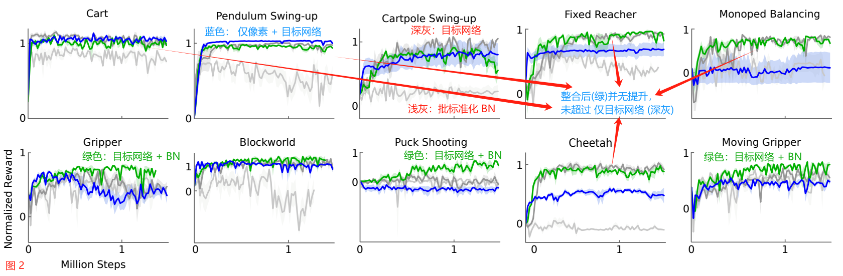
Figure 2: Performance curves for a selection of domains using variants of DPG: original DPG algorithm (minibatch NFQCA) with batch normalization (light grey), with target network (dark grey), with target networks and batch normalization (green), with target networks from pixel-only inputs (blue).
图 2：使用 DPG 变体选择域的性能曲线：
带有批标准化（浅灰色）的原始 DPG 算法（minibatch NFQCA），
带有目标网络（深灰色），带有目标网络和批标准化（绿色），带有纯像素输入的目标网络（蓝色）。
Target networks are crucial.
目标网络至关重要。

Surprisingly, in some simpler tasks, learning policies from pixels is just as fast as learning using the low-dimensional state descriptor.
令人惊讶的是，在一些更简单的任务中，从像素学习策略和使用低维状态描述符学习策略一样快。
This may be due to the action repeats making the problem simpler.
这可能是由于动作的重复使问题变得更简单。
It may also be that the convolutional layers provide an easily separable representation of state space, which is straightforward for the higher layers to learn on quickly.
也可能是卷积层提供了一种易于分离的状态空间表示，这对于更高的层来说是简单的，可以快速学习。

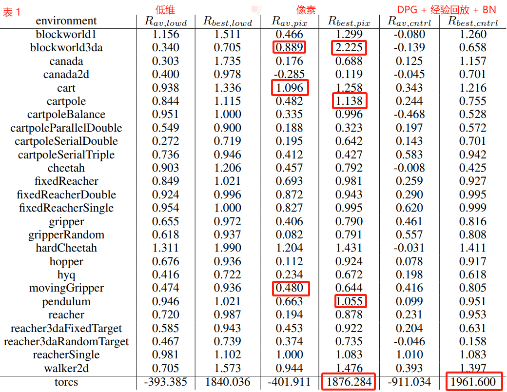
Table 1 summarizes DDPG’s performance across all of the environments (results are averaged over 5 replicas).
表 1 总结了 DDPG 在所有环境中的性能（结果是 5 个副本的平均值）。
We normalized the scores using two baselines.
我们使用两条基线将分数标准化。
The first baseline is the mean return from a naive policy which samples actions from a uniform distribution over the valid action space.
第一个基线是朴素策略的平均回报，该策略从有效动作空间的均匀分布中采样动作。
The second baseline is iLQG (Todorov & Li, 2005), a planning based solver with full access to the underlying physical model and its derivatives.
第二个基线是 iLQG (Todorov & Li, 2005)，这是一个基于规划的求解器，可以完全访问底层物理模型及其衍生物。
We normalize scores so that the naive policy has a mean score of 0 and iLQG has a mean score of 1.
我们将分数归一化，使朴素策略的平均分数为 0，iLQG 的平均分数为 1。
DDPG is able to learn good policies on many of the tasks, and in many cases some of the replicas learn policies which are superior to those found by iLQG, even when learning directly from pixels.
DDPG 能够在许多任务上学习良好的策略，并且在许多情况下，即使直接从像素学习，一些副本学习的策略也优于 iLQG 找到的策略。

Table 1: Performance after training across all environments for at most 2.5 million steps.
表 1：在所有环境中进行最多 250 万步的训练后的性能。
We report both the average and best observed (across 5 runs).
我们报告平均值和最佳观察值（跨越 5 次运行）。
All scores, except Torcs, are normalized so that a random agent receives 0 and a planning algorithm 1; for Torcs we present the raw reward score.
除 Torcs 外，所有分数都归一化，以便随机代理接收 0，规划算法接收 1；对于 Torcs，我们提供原始奖励分数。
We include results from the DDPG algorithn in the low-dimensional (lowd) version of the environment and high-dimensional (pix).
我们将 DDPG 算法的结果包含在低维（low）版本的环境和高维（pix）版本中。
For comparision we also include results from the original DPG algorithm with a replay buffer and batch normalization (cntrl).
为了进行比较，我们还包括原始 DPG 算法的结果，其中包含 replay buffer 和 batch normalization (cntrl)。

It can be challenging to learn accurate value estimates.
学习准确的价值估计是具有挑战性的。
Q-learning, for example, is prone to overestimating values (Hasselt, 2010).
We examined DDPG’s estimates empirically by comparing the values estimated by Q after training with the true returns seen on test episodes.
例如，Q-learning 容易高估值（Hasselt, 2010）。
我们通过比较训练后 Q 估计的值与测试集上看到的真实回报来检验 DDPG 的估计。
Figure 3 shows that in simple tasks DDPG estimates returns accurately without systematic biases.
图 3 显示，在简单的任务中，DDPG 准确地估计了回报，没有系统偏差。
For harder tasks the Q estimates are worse, but DDPG is still able learn good policies.
对于更难的任务，Q 估计更差，但 DDPG 仍然能够学习到好的策略。

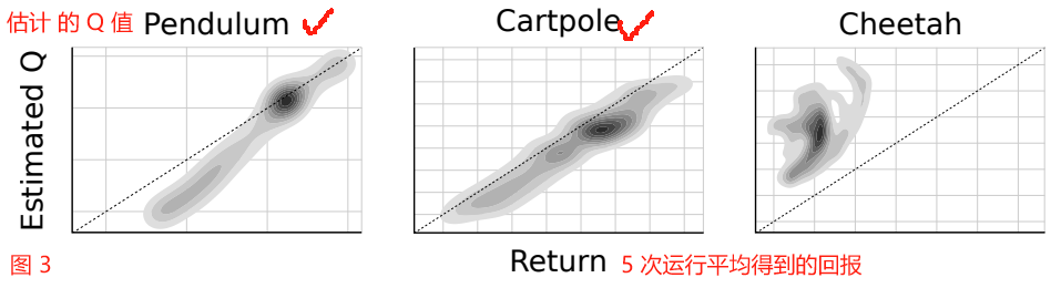
Figure 3: Density plot showing estimated Q values versus observed returns sampled from test episodes on 5 replicas.
图 3：密度图显示估计的 Q 值与 从 5 个副本的测试集中抽样观察到的回报。
In simple domains such as pendulum and cartpole the Q values are quite accurate.
在简单的领域，如 pendulum 和 cartpole ，Q 值是相当准确的。
In more complex tasks, the Q estimates are less accurate, but can still be used to learn competent policies.
在更复杂的任务中，Q 估计不太准确，但仍然可以用来学习有效的策略。
Dotted line indicates unity, units are arbitrary.
虚线表示统一，单位是任意的。

To demonstrate the generality of our approach we also include Torcs, a racing game where the actions are acceleration, braking and steering.
为了证明我们方法的通用性，我们还将 Torcs 纳入其中，这是一款赛车游戏，其中的动作是加速、刹车和转向。
Torcs has previously been used as a testbed in other policy learning approaches (Koutník et al., 2014b).
Torcs 此前已被用作其他策略学习方法的测试平台（Koutník等人，2014b）。
We used an identical network architecture and learning algorithm hyper-parameters to the physics tasks but altered the noise process for exploration because of the very different time scales involved.
我们对物理任务使用了相同的网络架构和学习算法超参数，但由于涉及的时间尺度非常不同，因此改变了探索的噪声过程。
On both low-dimensional and from pixels, some replicas were able to learn reasonable policies that are able to complete a circuit around the track though other replicas failed to learn a sensible policy.
在低维和像素上，一些副本能够学习到合理的策略，这些策略能够围绕赛道完成一个循环，而其他副本则无法学习到合理的策略。

5 相关工作

The original DPG paper evaluated the algorithm with toy problems using tile-coding and linear function approximators.
原始的 DPG 论文使用瓦片编码tile-coding 和线性函数近似器来评估玩具问题的算法。
It demonstrated data efficiency advantages for off-policy DPG over both on- and off-policy stochastic actor critic.
它证明了 off-policy DPG 在数据效率方面均优于on-policy 和 off-policy 随机 actor-critic。
It also solved one more challenging task in which a multi-jointed octopus arm had to strike a target with any part of the limb.
它还解决了另一个更具挑战性的任务，即多关节章鱼的手臂必须用肢体的任何部分击中目标。
However, that paper did not demonstrate scaling the approach to large, high-dimensional observation spaces as we have here.
然而，那篇论文并没有像我们在这里那样演示 将方法扩展到大的、高维的观察空间。

一个 tiling 的意思是一张大网，里面有划分成不同的小网，观察的像素会落到这个 tiling 中的小网内，就可以用这个小网内的坐标表示这个特征，多个 tiling 就是用多个小网内的坐标表示这个特征

It has often been assumed that standard policy search methods such as those explored in the present work are simply too fragile to scale to difficult problems (Levine et al., 2015).
人们通常认为，标准的策略搜索方法（如本工作中探索的方法）太脆弱，无法扩展到困难的问题（Levine et al., 2015）。
Standard policy search is thought to be difficult because it deals simultaneously with complex environmental dynamics and a complex policy.
标准策略搜索被认为是困难的，因为它同时处理复杂的环境动态和复杂的策略。
Indeed, most past work with actor-critic and policy optimization approaches have had difficulty scaling up to more challenging problems (Deisenroth et al., 2013).
事实上，大多数过去使用 actor-critic 和策略优化方法的工作都难以扩展到更具挑战性的问题（Deisenroth 等人，2013）。
Typically, this is due to instability in learning wherein progress on a problem is either destroyed by subsequent learning updates, or else learning is too slow to be practical.
通常，这是由于学习的不稳定性，其中问题的进展要么被随后的学习更新所破坏，要么学习太慢而无法实践。

Recent work with model-free policy search has demonstrated that it may not be as fragile as previously supposed.
最近对无模型策略搜索的研究表明，它可能不像以前想象的那么脆弱。
Wawrzyński (2009); Wawrzyński & Tanwani (2013) has trained stochastic policies in an actor-critic framework with a replay buffer.
Wawrzyński (2009); Wawrzyński & Tanwani (2013) 在带有 replay buffer 的 actor-critic 框架中训练了随机策略。
Concurrent with our work, Balduzzi & Ghifary(2015) extended the DPG algorithm with a “deviator” network which explicitly learns $\partial Q/\partial a$.
与我们的工作同时，Balduzzi 和 Ghifary（2015）用一个明确学习 $\partial Q/\partial a$ 的“偏差”网络扩展了 DPG 算法。
However, they only train on two low-dimensional domains.
然而，它们只在两个低维域上训练。
Heess et al. (2015) introduced SVG(0) whichalso uses a Q-critic but learns a stochastic policy.
Heess 等人（2015）引入了 SVG(0)，它也使用 Q-critic，但学习随机策略。
DPG can be considered the deterministic limit of SVG(0).
DPG 可认为是 SVG(0) 的确定性极限。
The techniques we described here for scaling DPG are also applicable to stochastic policiesby using the reparametrization trick (Heess et al., 2015; Schulman et al., 2015a).
我们在这里描述的缩放 DPG 的技术也适用于随机策略，通过使用重参数化技巧(Heess et al., 2015; Schulman et al., 2015a)。

Another approach, trust region policy optimization (TRPO) (Schulman et al., 2015b), directly constructs stochastic neural network policies without decomposing problems into optimal control and supervised phases.
另一种方法是 trust region policy optimization (TRPO) (Schulman et al., 2015b)，它直接构建随机神经网络策略，而不将问题分解为最优控制阶段和监督阶段。
This method produces near monotonic improvements in return by making carefully chosen updates to the policy parameters, constraining updates to prevent the new policy from diverging too far from the existing policy.
该方法通过对策略参数进行精心选择的更新，约束更新以防止新策略与现有策略偏离太远，从而产生接近单调的改进。
This approach does not require learning an action-value function, and (perhaps as a result) appears to be significantly less data efficient.
这种方法不需要学习动作价值函数，而且（可能因此）数据效率明显较低。

To combat the challenges of the actor-critic approach, recent work with guided policy search (GPS) algorithms (e.g., (Levine et al., 2015)) decomposes the problem into three phases that are relatively easy to solve: first, it uses full-state observations to create locally-linear approximations of the dynamics around one or more nominal trajectories, and then uses optimal control to find the locally-linear optimal policy along these trajectories; finally, it uses supervised learning to train a complex, non-linear policy (e.g. a deep neural network) to reproduce the state-to-action mapping of the optimized trajectories.
为了应对 actor-critic 方法的挑战，最近使用引导策略搜索（GPS）算法（例如，（Levine等人，2015））的工作将问题分解为相对容易解决的三个阶段：首先，它使用全状态观察来创建围绕一个或多个标称轨迹的动态的局部线性近似，然后使用最优控制来找到沿着这些轨迹的局部线性最优策略；最后，它使用监督学习来训练一个复杂的非线性策略（例如深度神经网络），以重现优化好的轨迹的状态到动作映射

This approach has several benefits, including data efficiency, and has been applied successfully to a variety of real-world robotic manipulation tasks using vision.
这种方法有几个好处，包括数据效率，并且已经成功地应用于使用视觉的各种现实世界的机器人操作任务。
In these tasks GPS uses a similar convolutional policy network to ours with 2 notable exceptions: 1. it uses a spatial softmax to reduce the dimensionality of visual features into a single (x, y) coordinate for each feature map, and 2. the policy also receives direct low-dimensional state information about the configuration of the robot at the first fully connected layer in the network.
在这些任务中，GPS 使用与我们相似的卷积策略网络，但有两个明显的例外：1. 它使用空间 softmax 将视觉特征的维数降低为每个特征映射的单个（x, y）坐标。
2. 该策略还接收关于网络中第一个完全连接层的机器人配置的直接低维状态信息。
Both likely increase the power and data efficiency of the algorithm and could easily be exploited within the DDPG framework.
两者都可能增加算法的性能和数据效率，并且可以很容易地在 DDPG 框架中利用。

PILCO (Deisenroth & Rasmussen, 2011) uses Gaussian processes to learn a non-parametric, probabilistic model of the dynamics.
PILCO （Deisenroth & Rasmussen, 2011）使用高斯过程来学习动力学的非参数概率模型。
Using this learned model, PILCO calculates analytic policy gradients and achieves impressive data efficiency in a number of control problems.
利用这个习得的模型，PILCO 计算分析策略梯度，并在许多控制问题中获得令人印象深刻的数据效率。
However, due to the high computational demand, PILCO is “impractical for high-dimensional problems” (Wahlström et al., 2015).
然而，由于高计算需求，PILCO 是“不适用于高维问题”（Wahlström et al., 2015）。
It seems that deep function approximators are the most promising approach for scaling reinforcement learning to large, high-dimensional domains.
深度函数近似器似乎是将强化学习扩展到大型高维域的最有前途的方法。

Wahlström et al. (2015) used a deep dynamical model network along with model predictive control to solve the pendulum swing-up task from pixel input.
Wahlström 等人（2015）使用深度动态模型网络以及模型预测控制来解决来自像素输入的钟摆摆动任务。
They trained a differentiable forward model and encoded the goal state into the learned latent space.
他们训练了一个可微前向模型，并将目标状态编码到习得的潜在空间中。
They use model-predictive control over the learned model to find a policy for reaching the target.
他们对习得的模型使用模型预测控制来找到达到目标的策略。
However, this approach is only applicable to domains with goal states that can be demonstrated to the algorithm.
然而，这种方法只适用于具有目标状态的领域，这些目标状态可以被算法证明。

Recently, evolutionary approaches have been used to learn competitive policies for Torcs from pixels using compressed weight parametrizations (Koutník et al., 2014a) or unsupervised learning (Koutník et al., 2014b) to reduce the dimensionality of the evolved weights.
最近，进化方法已被用于使用压缩权重参数化（Koutník 等人，2014a）或无监督学习（Koutník 等人，2014b）从像素中学习 Torcs 的有竞争力的策略，以降低进化权重的维数。
It is unclear how well these approaches generalize to other problems.
目前还不清楚这些方法如何推广到其他问题。

6 结论

The work combines insights from recent advances in deep learning and reinforcement learning, resulting in an algorithm that robustly solves challenging problems across a variety of domains with continuous action spaces, even when using raw pixels for observations.
这项工作结合了深度学习和强化学习最新进展的见解，产生了一种算法，即使在使用原始像素进行观察时，也能在具有连续动作空间的各种领域中健壮地解决具有挑战性的问题。
As with most reinforcement learning algorithms, the use of non-linear function approximators nullifies any convergence guarantees; however, our experimental results demonstrate that stable learning without the need for any modifications between environments.
与大多数强化学习算法一样，非线性函数近似器的使用使任何收敛保证无效；然而，我们的实验结果表明，稳定的学习不需要在环境之间进行任何修改。

Interestingly, all of our experiments used substantially fewer steps of experience than was used by DQN learning to find solutions in the Atari domain.
有趣的是，我们所有的实验都比 DQN 学习在 Atari 领域寻找解决方案所用的经验步少得多。
Nearly all of the problems we looked at were solved within 2.5 million steps of experience (and usually far fewer), a factor of 20 fewer steps than DQN requires for good Atari solutions.
我们所看到的几乎所有问题都是在 250 万步内解决的（通常更少），比 DQN 所需的优秀 Atari 解决方案少了 20 倍的步数。
This suggests that, given more simulation time, DDPG may solve even more difficult problems than those considered here.
这表明，给予更多的模拟时间，DDPG 可能解决比这里考虑的更困难的问题。

A few limitations to our approach remain.
我们的方法仍然存在一些限制。
Most notably, as with most model-free reinforcement approaches, DDPG requires a large number of training episodes to find solutions.
最值得注意的是，与大多数无模型强化方法一样，DDPG 需要大量的训练回合来找到解决方案。
However, we believe that a robust model-free approach may be an important component of larger systems which may attack these limitations (Gläscher et al., 2010).
然而，我们相信一个健壮的无模型方法可能是大型系统的一个重要组成部分，它可能会突破这些限制（Gläscher 等人，2010）。

参考文献

—— 补充信息

7 实验细节

我们使用 Adam （Kingma & Ba, 2014）学习神经网络参数，actor 和 critic 的学习率分别为 $10^{-4}$ 和 $10^{-3}$。
对于 Q，我们包括 L2 权重衰减 $10^{-2}$，并使用 $\gamma =0.99$ 的折扣因子。
对于软目标更新，我们使用的是 $\tau =0.001$。
神经网络对所有隐藏层使用校正非线性rectified non-linearity（Glorot et al., 2011）。〔 ReLU 〕
actor 的最终输出层是 tanh 层，用于绑定动作。
低维网络有 2 个隐藏层，分别有 400 和 300 个单元（≈ 130,000 个参数）。
直到 Q 的第二个隐藏层才包含动作。
当从像素学习时，我们使用了 3 个卷积层（没有池化），每层有 32 个过滤器。
接下来是两个全连接层，有 200 个单元（430,000 个参数）。
最后一层是 actor 和 critic 的权重和偏置分别从均匀分布 $[-3\times 10^{-3},3\times 10^{-3}]$ 和 $[3\times 10^{-4},3\times 10^{-4}]$ 对低维和像素情况进行初始化。
这是为了确保策略和价值估计的初始输出接近于零。
其他层从均匀分布初始化 $[-\frac{1}{\sqrt{f}},\frac{1}{\sqrt{f}}]$，其中 $f$ 是层的扇入。
直到全连接层才包含动作。
对于低维问题，我们训练的小批量大小为 64，像素为 16。
我们使用的 replay buffer 大小为 $10^6$。

For the exploration noise process we used temporally correlated noise in order to explore well in physical environments that have momentum.
对于探索噪声过程，我们使用了时间相关噪声，以便在具有动量的物理环境中进行探索。
We used an Ornstein-Uhlenbeck process (Uhlenbeck & Ornstein, 1930) with $\theta =0.15$ and $\sigma =0.2$.
我们使用了一个 Ornstein-Uhlenbeck 过程（Uhlenbeck ＆ Ornstein, 1930），其中 $\theta =0.15$，$\sigma =0.2$。
The Ornstein-Uhlenbeck process models the velocity of a Brownian particle with friction, which results in temporally correlated values centered around 0.
Ornstein-Uhlenbeck 过程模拟了带有摩擦的布朗粒子的速度，其结果是以 0 为中心的时间相关值。

8 规划算法

Our planner is implemented as a model-predictive controller (Tassa et al., 2012): at every time step we run a single iteration of trajectory optimization (using iLQG, (Todorov & Li, 2005)), starting from the true state of the system.
我们的规划器是作为模型预测控制器实现的（Tassa 等人，2012）：在每个时间步，我们从系统的真实状态开始运行一次轨迹优化迭代（使用 iLQG， （Todorov & Li, 2005））。
Every single trajectory optimization is planned over a horizon between 250ms and 600ms, and this planning horizon recedes as the simulation of the world unfolds, as is the case in model-predictive control.
每一个轨迹优化都是在 250ms 到 600ms 之间进行规划的，随着模拟世界的展开，这个规划范围会缩小，就像模型预测控制中的情况一样。

The iLQG iteration begins with an initial rollout of the previous policy, which determines the nominal trajectory.
iLQG 迭代从先前策略的初始试运行开始，该策略确定了标称轨迹。
We use repeated samples of simulated dynamics to approximate a linear expansion of the dynamics around every step of the trajectory, as well as a quadratic expansion of the cost function.
我们使用模拟动态的重复样本来近似轨迹每一步动态的线性展开，以及损失函数的二次展开。
We use this sequence of locally-linear-quadratic models to integrate the value function backwards in time along the nominal trajectory.
我们使用这个局部线性二次模型序列沿着标称轨迹在时间上向后积分价值函数。
This back-pass results in a putative modification to the action sequence that will decrease the total cost.
We perform a derivative-free line-search over this direction in the space of action sequences by integrating the dynamics forward (the forward-pass), and choose the best trajectory.
这种反向传递会导致对动作序列的假定修改，从而降低总成本。
我们在动作序列空间的这个方向上通过积分动态向前（forward-pass）执行无导数的直线搜索，并选择最佳轨迹。
We store this action sequence in order to warm-start the next iLQG iteration, and execute the first action in the simulator.
我们存储这个动作序列是为了预热启动下一个 iLQG 迭代，并在模拟器中执行第一个动作。
This results in a new state, which is used as the initial state in the next iteration of trajectory optimization.
这将产生一个新状态，作为下一次轨迹优化迭代的初始状态。

9 环境细节

9.1 Torcs 环境

For the Torcs environment we used a reward function which provides a positive reward at each step for the velocity of the car projected along the track direction and a penalty of -1 for collisions.
对于 Torcs 环境，我们使用了奖励函数，即在每一步中为汽车沿着轨道方向的速度提供正奖励，并为碰撞提供 -1 的惩罚。
Episodes were terminated if progress was not made along the track after 500 frames.
如果在 500 帧后没有沿着轨道前进，回合将被终止。

9.2 MuJoCo 环境

For physical control tasks we used reward functions which provide feedback at every step.
对于物理控制任务，我们使用奖励功能，在每一步提供反馈。
In all tasks, the reward contained a small action cost.
在所有任务中，奖励都包含一个小的动作损失。
For all tasks that have a static goal state (e.g. pendulum swing-up and reaching) we provide a smoothly varying reward based on distance to a goal state, and in some cases an additional positive reward when within a small radius of the target state.
对于所有具有静态目标状态的任务（例如，pendulum swing-up 和 reaching），我们根据到目标状态的距离提供平滑变化的奖励，并且在某些情况下，当在目标状态的小半径内时提供额外的正奖励。
For grasping and manipulation tasks we used a reward with a term which encourages movement towards the payload and a second component which encourages moving the payload to the target.
对于抓取和操控任务，我们使用了带有鼓励向有效载荷移动的项的奖励，以及鼓励将有效载荷移动到目标的第二个组件。
In locomotion tasks we reward forward action and penalize hard impacts to encourage smooth rather than hopping gaits (Schulman et al., 2015b).
在运动任务中，我们奖励向前动作并惩罚硬撞击，以鼓励平稳而不是跳跃的步态（Schulman 等人，2015b）。
In addition, we used a negative reward and early termination for falls which were determined by simple threshholds on the height and torso angle (in the case of walker2d).
此外，我们使用了负奖励和跌倒的提前终止，这是由高度和躯干角度的简单阈值决定的（在 walker2d 的情况下）。

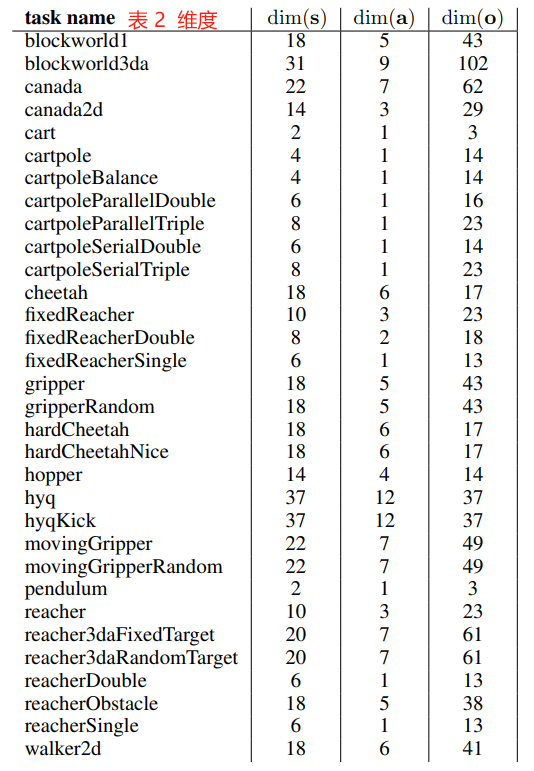
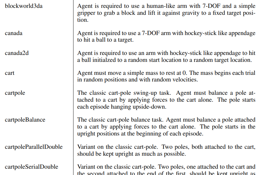
Table 2 states the dimensionality of the problems and below is a summary of all the physics environments.
表 2 列出了问题的维度，下面是对所有物理环境的总结。

Table 2: Dimensionality of the MuJoCo tasks: the dimensionality of the underlying physics model dim(s), number of action dimensions dim(a) and observation dimensions dim(o).
表 2： MuJoCo 任务的维度：底层物理模型的维度 dim(s)、动作的数量维度 dim(a) 和观察维度 dim(o) 。

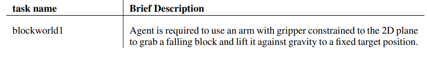
环境描述 部分