GoogLeNet论文解读—Going deeper with convolutions2015（V1）

GoogLeNet论文解读—Going deeper with convolutions2015

说明：本文只解读GooleNet的14年参赛的v1版本，之后的改进版本可能在日后的学习中继续更新

研究背景

更深的卷积神经网络

认识数据集：ImageNet的大规模图像识别挑战赛

LSVRC-2014：ImageNet Large Scale Visual Recoanition Challenge(14年的相关比赛)

ILSVRC：大规模图像识别挑战赛

ImageNet Large Scale Visual RecognitionChallenge是李飞飞等人于2010年创办的图像识别挑战赛，自2010起连续举办8年，极大地推动计算机视觉发展。

比赛项目涵盖：图像分类（Classification）、目标定位（Objectlocalization）、目标检测（Object detection）、视频目标检测（Object detection from video）、场景分类（Scene classification）、场景解析（Scenearsing）

竞赛中脱颖而出大量经典模型：
alexnet，vgg，googlenet，resnet，densenet

参考的研究背景：

1. NlN（NetworkinNetwork）：首个采用1*1卷积的卷积神经网络，舍弃全连接层，大大减少网络参数（网络中的网络）
2. Robust Object Recognition with Cortex-Like Mechanisms：多尺度Gabor滤波器提取特征
3. Hebbianprinciple（赫布理论 ）一起激发的神经元连接在一起

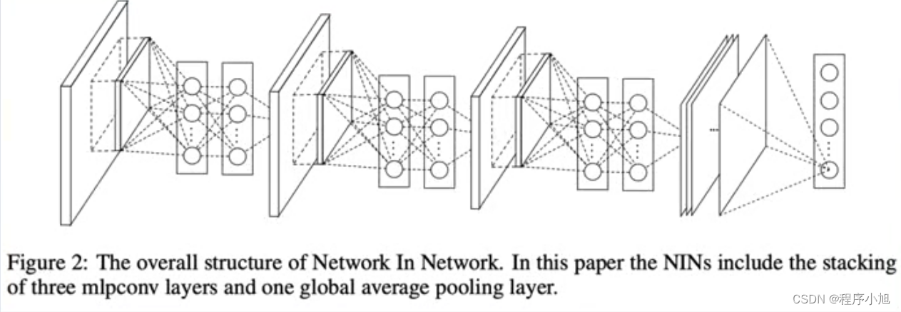
NiN网络

在李沐老师的动手学深度学习中有对NiN网络的相关的描述信息。
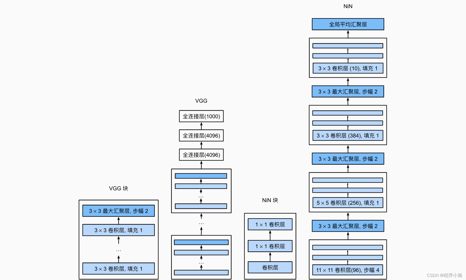
VGG和NiN及它们的块之间主要架构差异。 NiN块以一个普通卷积层开始，后面是两个的1x1卷积层。这两个卷积层充当带有ReLU激活函数的逐像素全连接层。 第一层的卷积窗口形状通常由用户设置。 随后的卷积窗口形状固定。

NIN(Network in Network):首个采用1 * 1卷积的卷积神经网络
特点：

• 1*1卷积
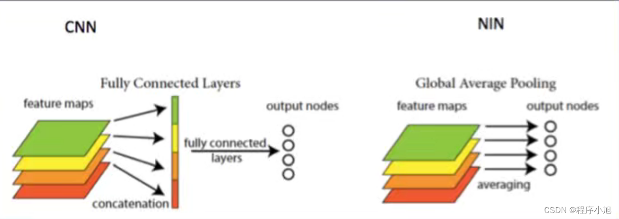
• GAP输出（全局平均池化）

回顾特征图输出大小的计算公式：

$$F_o=\lfloor \frac{F_{\text{in }}-k+2p}{s}\rfloor +1$$

对NIN中的数值进行分析可以得到的是在第一次我们采用的是224x224的三个通道的输入。

使用了11x11的步长为4的96个卷积核来进行卷积运算：应用公式可以得到：=（224-11）/4+1=54

得到了54x54的96通道数的输出值（与Alexnet保持相同）

之后使用3x3的maxpooling 步长为2(不改变通道数)

=（54-3）/2+1 =26

之后就得到了26x26x96的输出，中间的nin块使用了两个全连接的卷积层来代替全连接层

之后的分析过程相同，可以理解为在AlexNet的基础上引入了1x1的卷积核

研究成果

GoogLeNet：

分类第一名，检测第一名 ，定位第二名

VGG：定位第一名，分类第二名

1. 开启多尺度卷积时代
2. 拉开1*1卷积广泛应用序幕
3. 为GoogLeNet系列开辟道路（v1-v2-v3-v4）

论文精读

摘要

We propose a deep convolutional neural network architecture codenamed Inception, which was responsible for setting the new state of the art for classification and detection in the ImageNet Large-Scale Visual Recognition Challenge 2014(ILSVRC14). The main hallmark of this architecture is the improved utilization of the computing resources inside the network. This was achieved by a carefully crafted design that allows for increasing the depth and width of the network while keeping the computational budget constant. To optimize quality, the architectural decisions were based on the Hebbian principle and the intuition of multi-scale processing. One particular incarnation used in our submission for ILSVRC14 is called GoogLeNet, a 22 layers deep network, the quality of which is assessed in the context of classification and detection.

摘要总结：

1. 本文主题：提出名为lnception的深度卷积神经网络，在ILSVRC-2014获得分类及检测双料冠军
2. 模型特点1：Inception特点是提高计算资源利用率，增加网络深度和宽度时，参数少量增加
3. 模型特点2：借鉴Hebbain理论和多尺度处理

论文结构

1. introduction
2. RelatedWork
3. Motivation and High Level Considerations
4. ArchitecturalDetails
5. GoogLeNet
6. Trainning ethodology
7. ILSVRC 2014 Classification Challenge Setup and Results
8. ILSVRC 2014 Detection Challenge Setup and Results
9. Conclusions
10. Acknowlegements

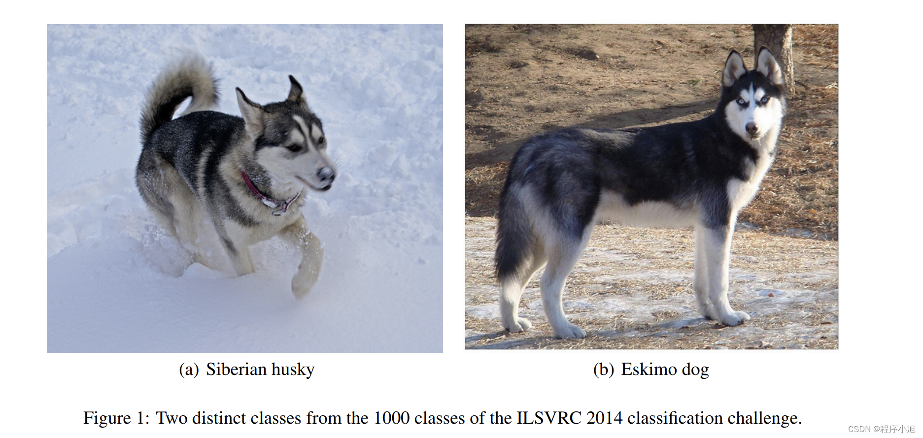
论文中的图一任务：举例说明了分类任务本身就是比较有难度的，哈士奇犬和爱斯基摩犬本身就难以区分。

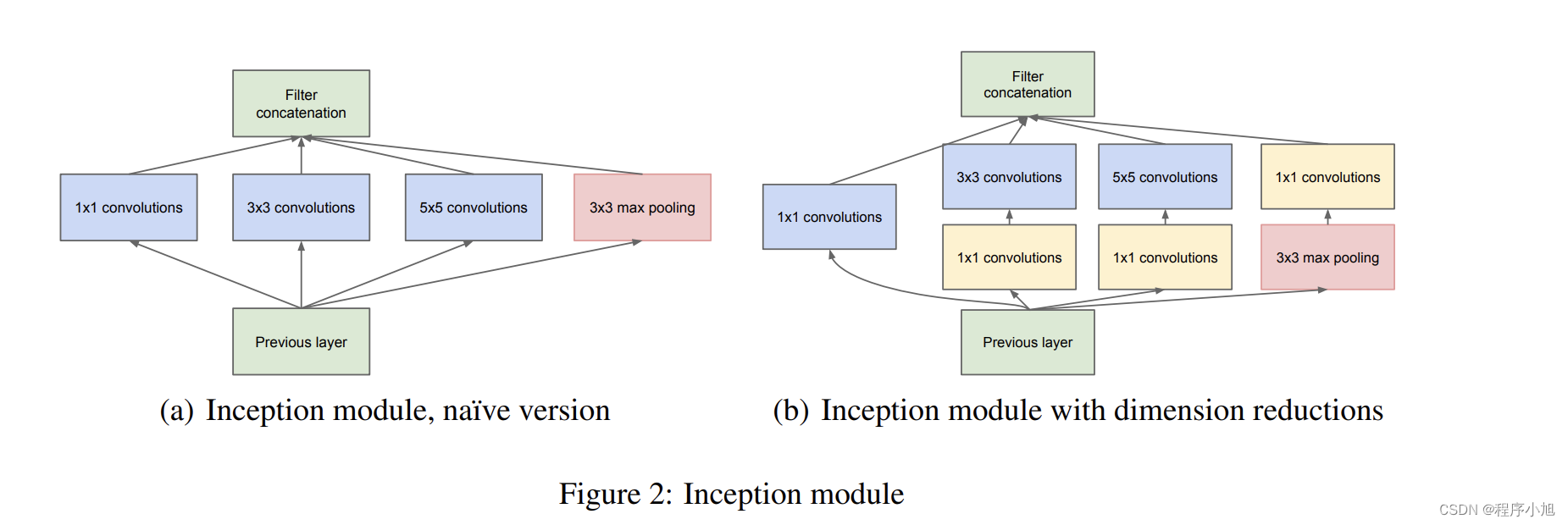
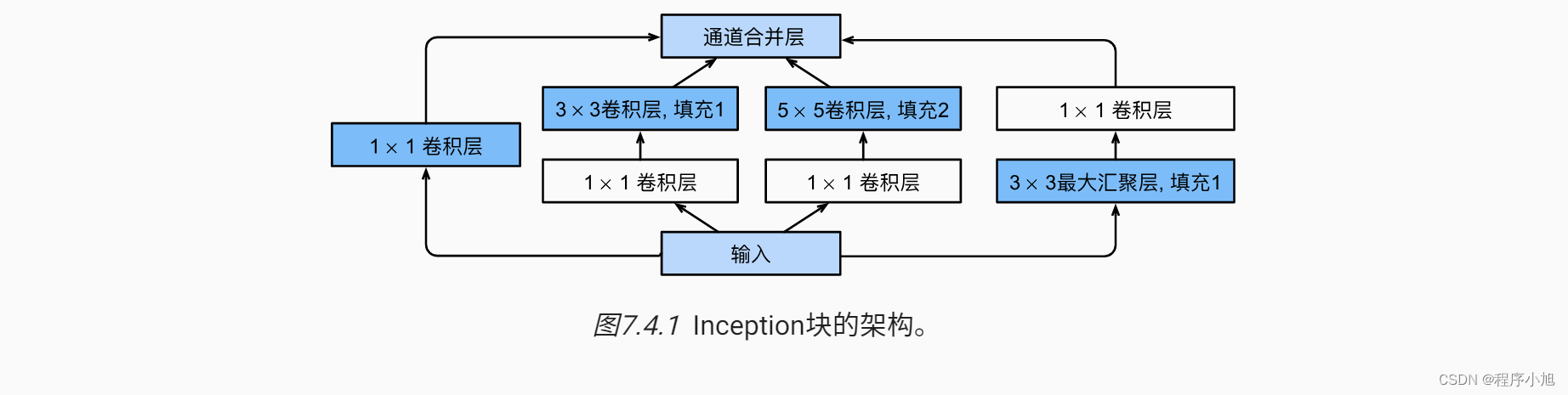
论文中的图二任务解释了多尺度卷积的inception结构，和其改进之后的形式。（补充动手学深度学习中的图）

GoogLenet网络结构

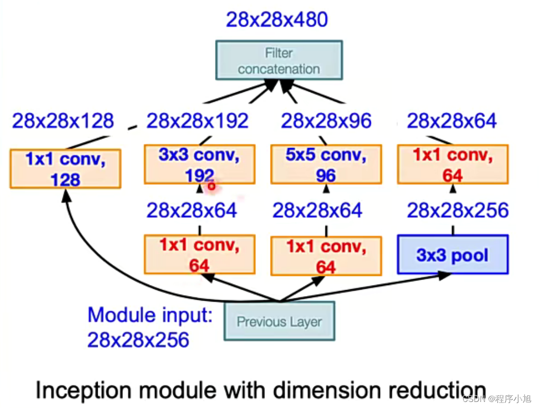
Inception Module

特点：

1. 多尺度
2. 1*1卷积降维，信息融合
3. 3*3 max pooling 保留了特征图数量

图片中的改进方式主要体现在了降维上

首先说明之前的Inception Module存在的问题

结合原始的inception结构（3x3的填充为1 5x5的填充为2,可以使得输出的大小保持不变28x28）

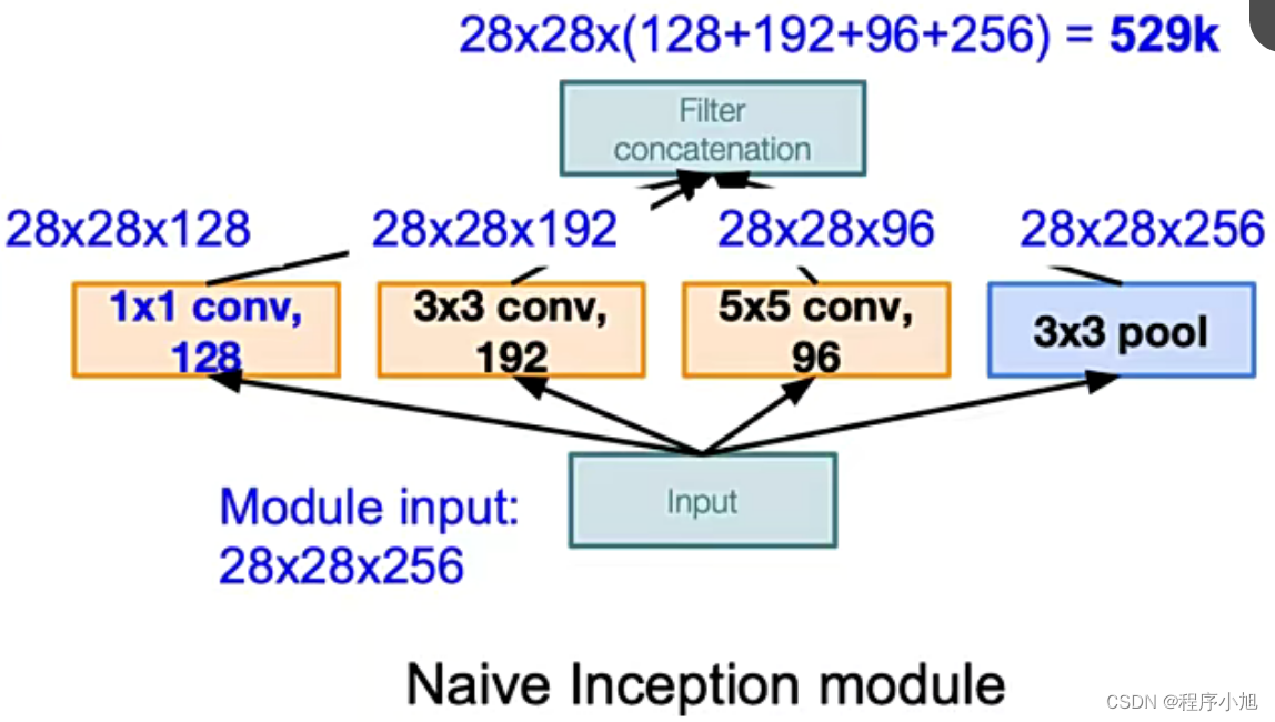
最后几个尺度得到的特征图都是28x28在融合的过程中将通道数进行相加运算。

3 * 3pool可让特征图通道数增加，且用较少计算量。缺点：数据量激增

其中计算量大的主要的原因是因为通道数过多导致了，计算的参数量过大，解决的办法就是使用1x1卷积进行一个通道融合的操作

主要的降维解决方法如下:

首先3x3的pooling还保留了原来的256个通道数，使用1x1的卷积核进行降维处理，保持64个通道数，在3x3卷积核与5x5卷积核在28x28x256上进行卷积的运算量过多，使用1x1的64卷积核对特征进行了一部分的压缩处理

$$F_i\times \left(K_{\mathrm{s}}\times K_{\mathrm{s}}\right)\times K_n+K_n$$

Fi:输入的通道数
ks：卷积核的尺寸
kn:卷积核的数量（输出的通道数）

Fi从256到64减少参数的运算

网络架构

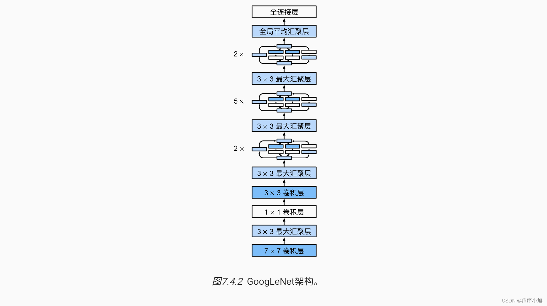
1. 三阶段：conv-pool-conv-pool快速降低分辨率；堆叠lnception；FC层分类输出
2. 堆叠使用lnceptionModule，达22层
3. 增加两个辅助损失，缓解梯度消失（中间层特征具有分类能力）

简化之后的网络结构可以用动手学深度学习中的图来进行简化操作

而论文中也给出了表格形式的具体的描述信息：

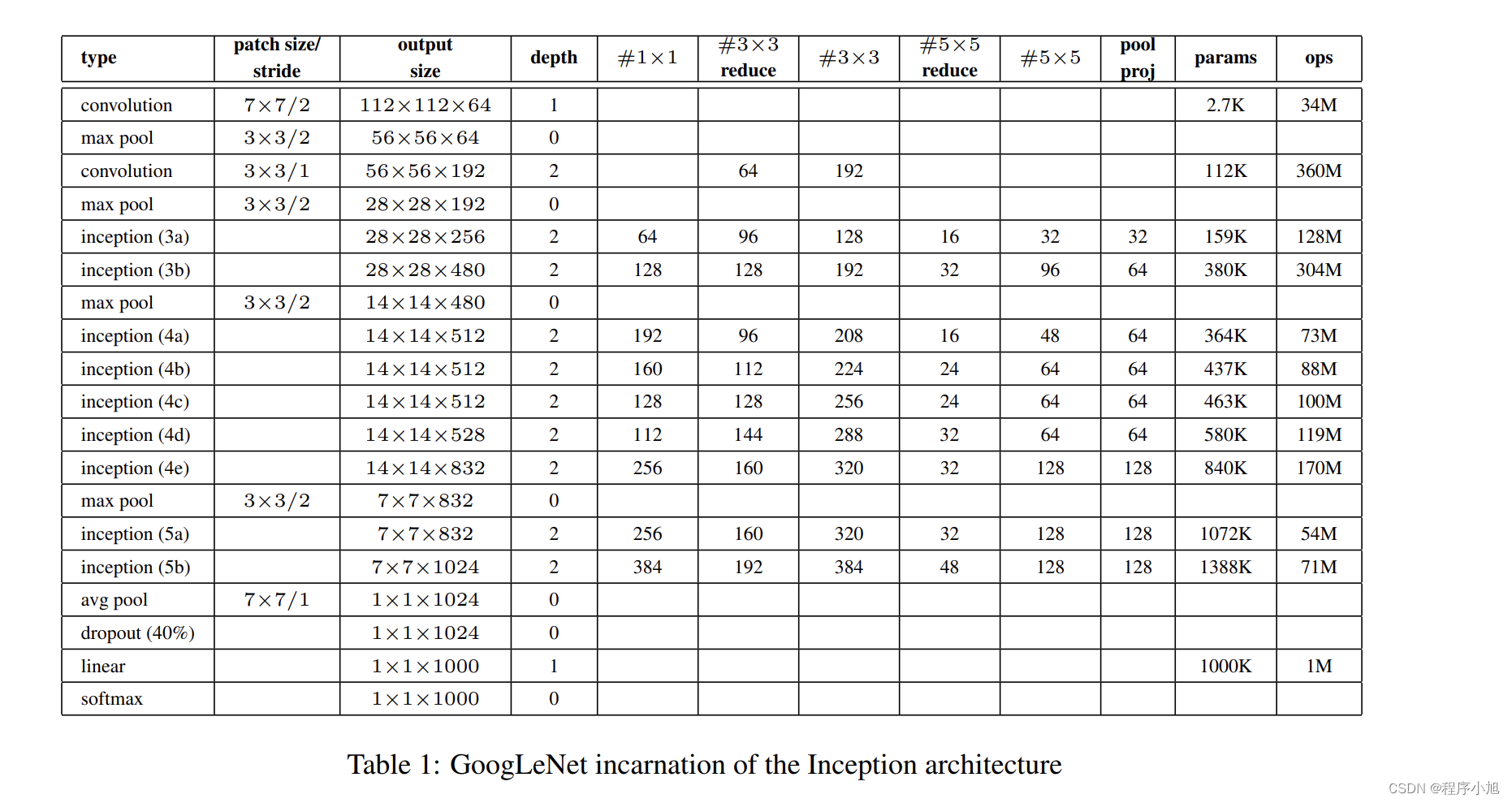
根据这个图表中给出的参数，简单解释一下计算的步骤，同样输入的图片也是224x224的3通道彩色图像。

首先进行7x7的步长为2的卷积运算（padding=3做减半运算）

=（224-7+6）/2 +1=112
第二次池化的padding=1做减半运算
=（112+2-1）/2 +1 =56

之后的运算过程结合公式依次进行类推。（设置的参数之间并没有发现一些规律）

All the convolutions, including those inside the Inception modules, use rectified linear activation.
The size of the receptive field in our network is 224×224 taking RGB color channels with mean subtraction. “#3×3 reduce” and “#5×5 reduce” stands for the number of 1×1 filters in the reduction
layer used before the 3×3 and 5×5 convolutions. One can see the number of 1×1 filters in the projection layer after the built-in max-pooling in the pool proj column. All these reduction/projection
layers use rectified linear activation as well.
The network was designed with computational efficiency and practicality in mind, so that inference
can be run on individual devices including even those with limited computational resources, especially with low-memory footprint. The network is 22 layers deep when counting only layers with
parameters (or 27 layers if we also count pooling). The overall number of layers (independent building blocks) used for the construction of the network is about 100. However this number depends on
the machine learning infrastructure system used. The use of average pooling before the classifier is
based on [12], although our implementation differs in that we use an extra linear layer. This enables
adapting and fine-tuning our networks for other label sets easily, but it is mostly convenience and
we do not expect it to have a major effect. It was found that a move from fully connected layers to
average pooling improved the top-1 accuracy by about 0.6%, however the use of dropout remained
essential even after removing the fully connected layers.

训练技巧（Training Tricks）

辅助损失（训练使用）

在lnception4b和Inception4e增加两个辅助分类层，用于计算辅助损失
达到

1. 增加loss回传
2. 充当正则约束，迫使中间层特征也能具备分类能力

后面的后续论文中证明了辅助损失几乎没什么作用

数据增强

指导方针：

1. 图像尺寸均匀分布在8%-100%之间
2. 长宽比在[3/4，4/3]之间
3. Photometricdistortions有效，如亮度、饱和度和对比度等

论文原文中（第6部分）没有公布具体的训练方法，对于数据增强的方式，描述入下：

so it is hard to give a definitive guidance to the most effective single way to train these networks.

To complicate matters further, some of the models were mainly trained on smaller relative crops, others on larger ones, inspired by [8]. Still, one prescription that was verified to work very well after the competition includes sampling of various sized patches of the image whose size is distributed evenly between 8% and 100% of the image area and whose aspect ratio is chosen randomly between 3/4 and 4/3. Also, we found that the photometric distortions by Andrew Howard [8] were useful to combat overfitting to some extent. In addition, we started to use random interpolation methods (bilinear, area, nearest neighbor and cubic, with equal probability) for resizing relatively late and in conjunction with other hyperparameter changes, so we could not tell definitely whether the final results were affected positively by their use.

测试技巧

1. Multi crop（不是特别理解简单理解为防止过拟合的一种数据增强方式）文章将 1张图变144张图

• Step1：等比例缩放短边至256，288，320，352，四种尺寸。一分为四
• Step2：在长边上裁剪出3个正方形，左中右或者上中下，三个位置。一分为三
• Step3:左上，右上，左下，右下，中心，全局resize，六个位置。一分为六
• Step4：水平镜像。一分为二
• 436*2=144

2. 原文中提到了模型融合的概念

1. We independently trained 7 versions of the same GoogLeNet model (including one wider
   version), and performed ensemble prediction with them. These models were trained with
   the same initialization (even with the same initial weights, mainly because of an oversight)
   and learning rate policies, and they only differ in sampling methodologies and the random
   order in which they see input images

七个模型训练差异仅在图像采样方式和顺序的差异(超参数的不同)

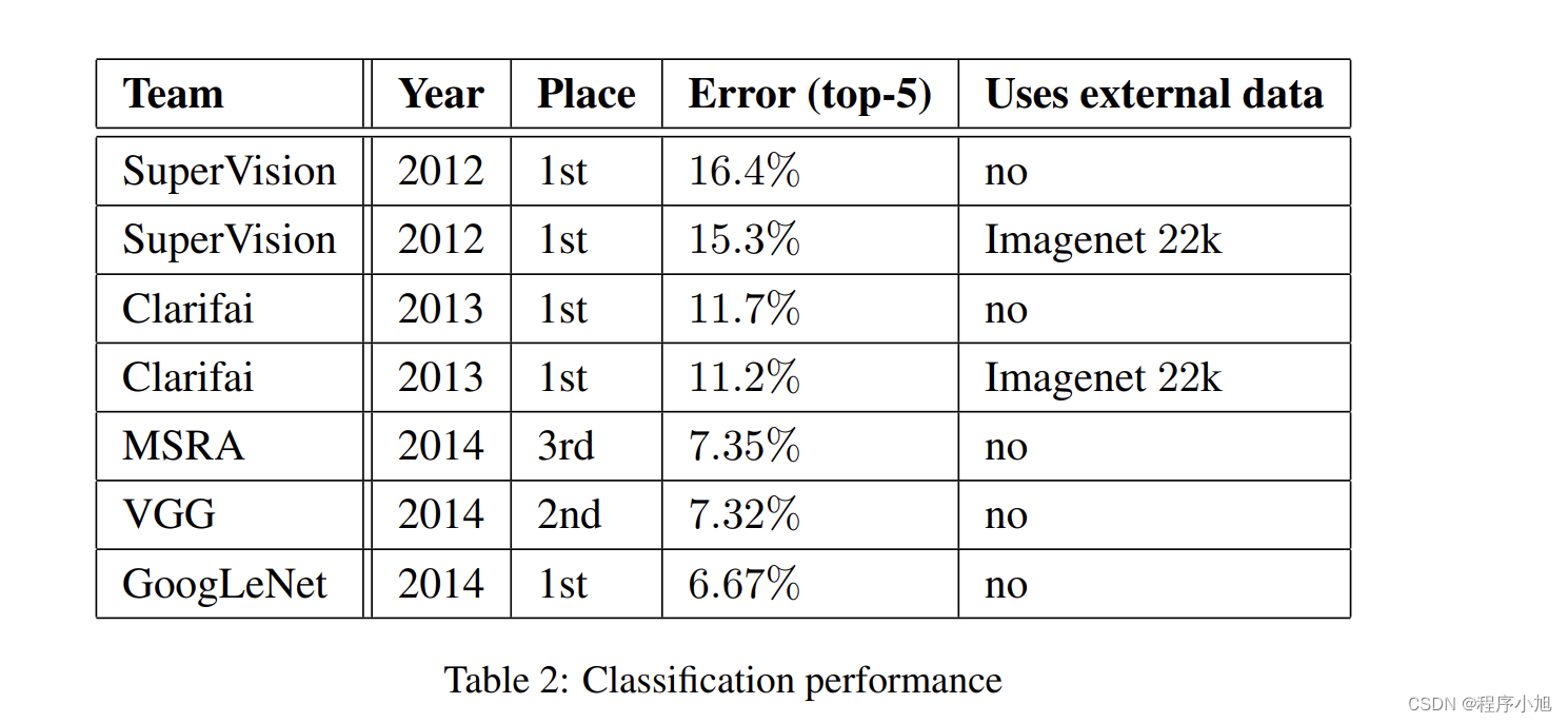
结合测试的模型实验值

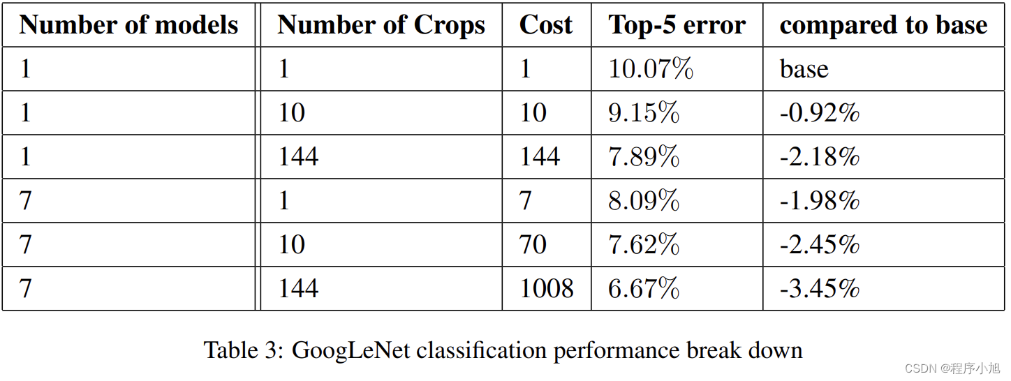
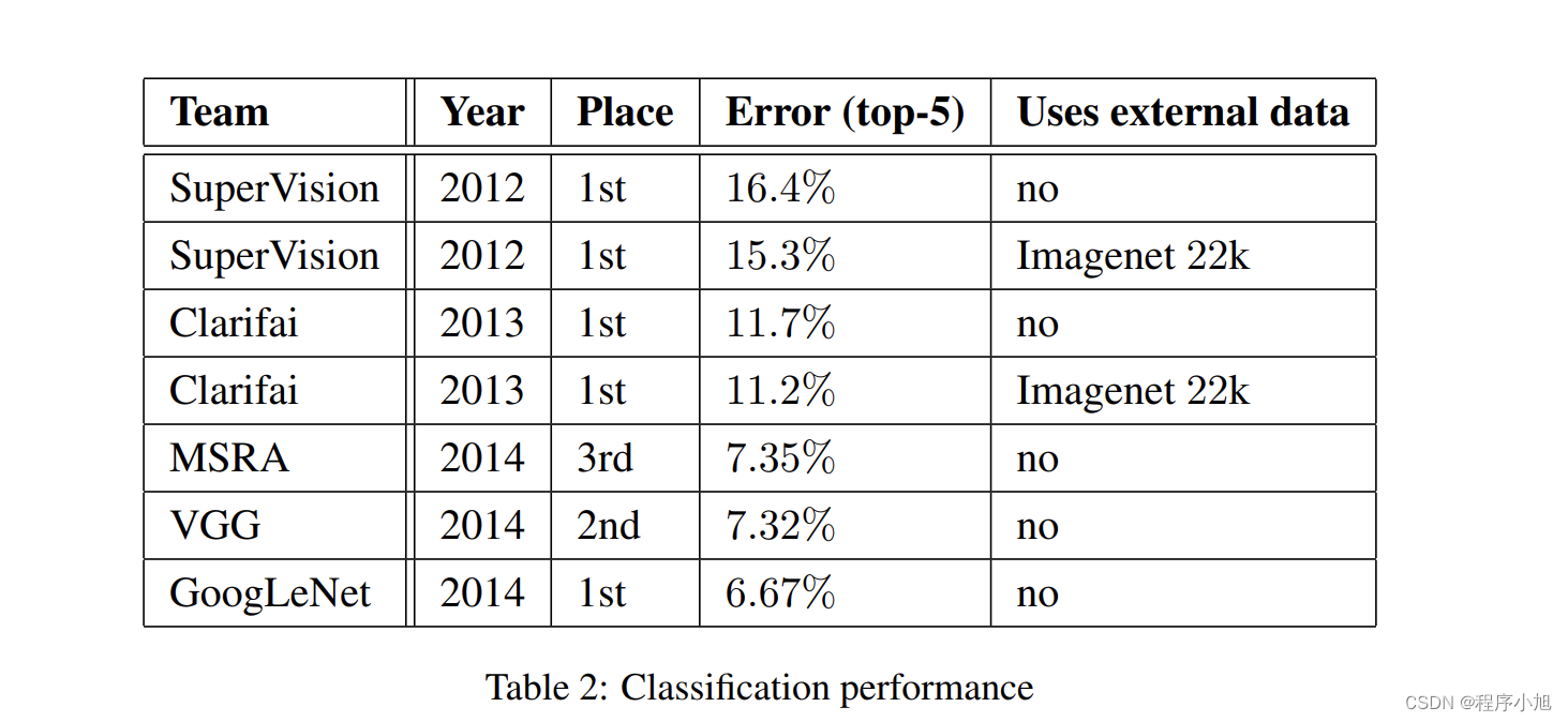
单模型的效果一般，多模型的效果更好