2*2子图/空间插值图/ax平移

# -*- coding: utf-8 -*-

import numpy as np
import shapefile
from shapely.geometry import Polygon
from shapely.ops import unary_union
import cartopy.io.shapereader as shpreader
import cartopy.crs as ccrs
from matplotlib.path import Path
from matplotlib.patches import PathPatch
import matplotlib.pyplot as plt
from scipy.interpolate import Rbf
import netCDF4 as nc

plt.rcParams['font.family'] = 'Times New Roman, SimSun'  # 设置字体族，中文为SimSun，英文为Times New Roman
plt.rcParams['mathtext.fontset'] = 'stix'  # 设置数学公式字体为stix


def draw_ax_function(ax, path0, lon, lat, value, text1, text2):
    file = shapefile.Reader(path0)
    rec = file.shapeRecords()
    polygon = list()
    for r in rec:
        polygon.append(Polygon(r.shape.points))
    poly = unary_union(polygon)  # 并集
    ext = list(poly.exterior.coords)  # 外部点
    codes = [Path.MOVETO] + [Path.LINETO] * (len(ext) - 1) + [Path.CLOSEPOLY]
    #    codes += [Path.CLOSEPOLY]
    ext.append(ext[0])  # 起始点
    path = Path(ext, codes)
    patch = PathPatch(path, facecolor='None')

    xi = np.arange(115.4, 117.5, 0.01)
    yi = np.arange(39.4, 41.2, 0.01)
    olon, olat = np.meshgrid(xi, yi)

    # Rbf空间插值
    func = Rbf(lon, lat, value, function='linear')
    oz = func(olon, olat)
    ax.add_patch(patch)
    rain_levels = [0, 0.1, 10, 25, 50, 100, 250, 25000]
    rain_colors = ['#FFFFFF', '#A6F28F', '#38A800', '#61B8FF', '#0000FF', '#FA00FA', '#730000', '#400000']
    pic = ax.contourf(olon, olat, oz, levels=rain_levels, colors=rain_colors)
    for collection in pic.collections:
        collection.set_clip_path(patch)  # 设置显示区域

    # 添加地市边界
    # ax.add_geometries(shp, ccrs.PlateCarree(), edgecolor='black',
    #                   facecolor='none', alpha=0.3, linewidth=0.5)  # 加底图

    ax.axis('off')  # 去除四边框框
    # 图例
    position = fig.add_axes([0.2, 0.08, 0.6, 0.03])  # 位置
    cbar = plt.colorbar(pic, ticks=[0, 0.1, 10, 25, 50, 100, 250], cax=position, orientation="horizontal")
    cbar.set_label('mm')  #
    # 添加标注
    ax.text(0, 0.9, text1, transform=ax.transAxes, size=13)
    ax.text(0.3, -0.1, text2, transform=ax.transAxes, size=13)


if __name__ == '__main__':
    dataset = nc.Dataset('data.nc')  # 读取数据
    print(dataset.variables.keys())  # 输出所有变量
    lon = dataset.variables['longitude'][:].data  # 读取经度,461-471
    lat = dataset.variables['latitude'][:].data  # 读取维度,196-203
    time = dataset.variables['time']  # 读取时间,112-232
    real_time = nc.num2date(time, time.units).data.reshape(-1, 1)  # 转成时间格式
    tp = dataset.variables['tp'][:].data * 1000
    beijin_tp = tp[112:233 - 6, 196:204, 461:472]
    beijin_lon = lon[461:472]
    beijin_lat = lat[196:204]
    lons, lats = np.meshgrid(beijin_lon, beijin_lat)
    # 画图
    titles = ['(a)7月29日00-06时', '(b)7月29日06-12时', '(c)7月29日12-18时', '(d)7月29日18-24时',
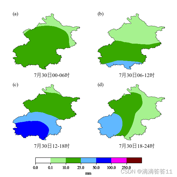
              '(a)7月30日00-06时', '(b)7月30日06-12时', '(c)7月30日12-18时', '(d)7月30日18-24时',
              '(a)7月31日00-06时', '(b)7月31日06-12时', '(c)7月31日12-18时', '(d)7月31日18-24时',
              '(a)8月1日00-06时', '(b)8月1日06-12时', '(c)8月1日12-18时', '(d)8月1日18-24时',
              '(a)8月2日00-06时', '(b)8月2日06-12时', '(c)8月2日12-18时', '(d)8月2日18-24时']

    path0 = r"beijin\beijin.shp"
    num = 0
    for step in range(5):
        fig, ((ax1, ax2), (ax3, ax4)) = plt.subplots(nrows=2, ncols=2, figsize=(6, 6))
        ax1.set_position([0.07, 0.6, 0.4, 0.35])
        ax2.set_position([0.55, 0.6, 0.4, 0.35])
        ax3.set_position([0.07, 0.2, 0.4, 0.35])
        ax4.set_position([0.55, 0.2, 0.4, 0.35])
        print(step)
        for i, ax, in zip(range(step * 4, step * 4 + 4), [ax1, ax2, ax3, ax4]):
            title = titles[num]
            draw_ax_function(ax, path0, lons.reshape(-1, 1), lats.reshape(-1, 1),
                             np.sum(beijin_tp[i * 6:i * 6 + 6, :, :], 0).reshape(-1, 1), title[:3], title[3:])
            num = num + 1
        plt.savefig(str(step) + '.png')
    # 显示图像
    plt.show()

效果图如下: