机器学习_5机器学习库Scikit-learn

本博文基于温州大学黄海广机器学习慕课（https://www.icourse163.org/learn/WZU-1464096179?tid=1466943454#/learn/announce）进行知识梳理。

Scikit-learn概述

包括分类、回归、降维、聚类四大机器学习算法；包括特征提取、数据处理、模型评估三大模块。

Scikit-learn主要用法

符号标记：

无监督学习的话就没有标签（y）

基本建模流程

• 导入工具包

from sklearn import datasets,preprocessing
from sklearn.model_selection import train_test_split
from sklearn.linear_model import LinerRegression(线性回归）
from sklearn.metrics import r2_score

• 加载数据
  支持Numpy的arrays对象、Pandas对象、SciPy的稀疏矩阵及其他可转换为数值型arrays的数据结构。数据必须是数值型的。
  提供了一系列加载和获取著名数据集，如鸢尾花（分类）、波士顿房价（回归）、Olivetti人脸（人脸识别）、MNIST（图像）数据集等的工具。

# 鸢尾花数据集
from sklearn.datasets import load_iris
iris=load_iris()
X=iris.data
y=iris.target

• 数据划分

from sklearn.model_selection import train_test_split
X_train,X_test,y_train,y_test=train_test_split(X,y,random_state=12,stratify=y,test_size=0.3)
# 70%作为训练集，30%作为测试集；stratify=y表示各类别数据的比例与原始数据集比例一致；可通过shuffle=True提前打乱数据。（随机性大些）

• 数据预处理

# 使用Scikit_learn进行数据标准化
from sklearn.preprocessing import StandardScaler
# 构建转换器实例
scaler=StandardScaler()
# 拟合及转换
scaler.fit_transform(X_train)

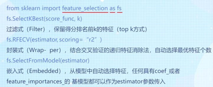
• 特征选择
  

监督学习算法

回归

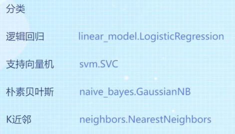
分类

clf 一般代表分类器；max_depth 具体的参数；y_pred 直接预测出属于哪一类；y_prob直接预测出概率。

集成学习

无监督学习算法

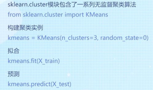
聚类

评价指标

accuracy_score 准确率：y_true真实标签/y_pred预测标签

回归的评价指标

用法：y_true真实标签 和 y_pred预测标签 带入

分类的评价指标

超参数调优

交叉验证

网格搜索——速度非常慢

随机搜索

Scikit-learn案例代码实现

建立简单机器学习的方法

在数据集上训练和测试一个分类器。划分数据后，使用fit方法学习机器学习模型，使用score方法测试此方法依赖于默认的准确度指标。

import matplotlib.pyplot as plt
from sklearn.datasets import load_digits
X, y = load_digits(return_X_y=True)
print(X.shape) # (1797, 64)
# X中的每行包含64个图像像素的强度。 对于X中的每个样本，我们得到表示所写数字对应的y。
# 绘制灰度图
plt.imshow(X[0].reshape(8, 8), cmap='gray')# 灰度显示图像
plt.axis('off')# 关闭坐标轴
print('The digit in the image is {}'.format(y[0]))# 格式化打印
plt.show()

# 划分数据
from sklearn.model_selection import train_test_split
X_train, X_test, y_train, y_test = train_test_split( X, y, stratify=y, test_size=0.25, random_state=42)
# 划分数据为训练集与测试集,添加stratify参数使得训练和测试数据集的类分布与整个数据集的类分布相同。

from sklearn.linear_model import LogisticRegression  # 求出Logistic回归的精确度得分
clf = LogisticRegression(solver='lbfgs', multi_class='ovr', max_iter=5000, random_state=42)
clf.fit(X_train, y_train)
accuracy = clf.score(X_test, y_test)
print('Accuracy score of the {} is {:.4f}'.format(clf.__class__.__name__, accuracy))
# Accuracy score of the LogisticRegression is 0.9622

from sklearn.ensemble import RandomForestClassifier
# RandomForestClassifier轻松替换LogisticRegression分类器
clf = RandomForestClassifier(n_estimators=1000, n_jobs=-1, random_state=42)
clf.fit(X_train, y_train)
accuracy = clf.score(X_test, y_test)
print('Accuracy score of the {} is {:.2f}'.format(clf.__class__.__name__, accuracy))
# Accuracy score of the RandomForestClassifier is 0.97

from xgboost import XGBClassifier
clf = XGBClassifier(n_estimators=1000)
clf.fit(X_train, y_train)
accuracy = clf.score(X_test, y_test)
print('Accuracy score of the {} is {:.2f}'.format(clf.__class__.__name__, accuracy))
# Accuracy score of the XGBClassifier is 0.96

from sklearn.ensemble import GradientBoostingClassifier
clf = GradientBoostingClassifier(n_estimators=100, random_state=0)
clf.fit(X_train, y_train)
accuracy = clf.score(X_test, y_test)
print('Accuracy score of the {} is {:.2f}'.format(clf.__class__.__name__,accuracy))
# Accuracy score of the GradientBoostingClassifier is 0.96
from sklearn.metrics import balanced_accuracy_score
y_pred = clf.predict(X_test)
accuracy = balanced_accuracy_score(y_pred, y_test)
print('Accuracy score of the {} is {:.2f}'.format(clf.__class__.__name__, accuracy))
# Accuracy score of the GradientBoostingClassifier is 0.96

from sklearn.svm import SVC
clf = SVC()
clf.fit(X_train, y_train)
accuracy = clf.score(X_test, y_test)
print('Accuracy score of the {} is {:.2f}'.format(clf.__class__.__name__,accuracy))
# Accuracy score of the SVC is 0.99

from sklearn.svm import LinearSVC
clf = LinearSVC()
clf.fit(X_train, y_train)
accuracy = clf.score(X_test, y_test)
print('Accuracy score of the {} is {:.2f}'.format(clf.__class__.__name__,accuracy))
# Accuracy score of the LinearSVC is 0.93

数据预处理

规范化数据

from sklearn.datasets import load_digits
X, y = load_digits(return_X_y=True)
# 划分数据
from sklearn.model_selection import train_test_split
X_train, X_test, y_train, y_test = train_test_split( X, y, stratify=y, test_size=0.25, random_state=42)
# 划分数据为训练集与测试集,添加stratify参数使得训练和测试数据集的类分布与整个数据集的类分布相同。

from sklearn.preprocessing import MinMaxScaler # 归一化数据
from sklearn.svm import LinearSVC
scaler = MinMaxScaler()
X_train_scaled = scaler.fit_transform(X_train) # 标准用法
X_test_scaled = scaler.transform(X_test) # 标准用法
clf = LinearSVC()
clf.fit(X_train_scaled, y_train)
accuracy = clf.score(X_test_scaled, y_test)
print('Accuracy score of the {} is {:.2f}'.format(clf.__class__.__name__,accuracy))
# Accuracy score of the LinearSVC is 0.97

from sklearn.preprocessing import StandardScaler  # 标准化数据
scaler = StandardScaler()
X_train_scaled = scaler.fit_transform(X_train)
X_test_scaled = scaler.transform(X_test)
clf = LinearSVC()
clf.fit(X_train_scaled, y_train)
accuracy = clf.score(X_test_scaled, y_test)
print('Accuracy score of the {} is {:.2f}'.format(clf.__class__.__name__,accuracy))
# Accuracy score of the LinearSVC is 0.95

错误的规范化方式：

• 未切分数据之前就做了规范化
• 独立的标准化训练集和测试集（都用了fit_transform)，造成数据分布不一致。
  正确的用法：

X_train_scaled = scaler.fit_transform(X_train) # 标准用法
X_test_scaled = scaler.transform(X_test) # 标准用法

管道连接器_流水线方法

规范化数据会产生数据泄露的问题，引入Pipeline对象，导入管道流水线，依次连接多个转换器和分类器（或回归器）。

from sklearn.datasets import load_digits
X, y = load_digits(return_X_y=True)
# 划分数据
from sklearn.model_selection import train_test_split
X_train, X_test, y_train, y_test = train_test_split( X, y, stratify=y, test_size=0.25, random_state=42)
# 划分数据为训练集与测试集,添加stratify参数使得训练和测试数据集的类分布与整个数据集的类分布相同。

from sklearn.preprocessing import MinMaxScaler
from sklearn.linear_model import LogisticRegression
from sklearn.pipeline import Pipeline
pipe=Pipeline(steps=[('scaler',MinMaxScaler()),
                     ('clf',LogisticRegression(solver='lbfgs',multi_class='auto',random_state=42))])
                     
pipe.fit(X_train,y_train)
accuracy=pipe.score(X_test,y_test)
print('Accuracy score of the {} is {:.2f}'.format(pipe.__class__.__name__,accuracy))
# Accuracy score of the Pipeline is 0.96

管道包含了归一化和分类器的参数，但有时，为管道中的每个估计器命名会很繁琐，make_pipeline将自动为每个估计器命名。

from sklearn.pipeline import make_pipeline
pipe=make_pipeline(MinMaxScaler(),LogisticRegression(solver='lbfgs',multi_class='auto',random_state=42,max_iter=1000))

检查管道的所有参数get_params()

clf.get_params()
pipe.get_params()
grid.get_params()

上述采用：

print(pipe.get_params())
# {'memory': None, 'steps': [('minmaxscaler', MinMaxScaler()), ('logisticregression', LogisticRegression(max_iter=1000, random_state=42))],
# 'verbose': False, 'minmaxscaler': MinMaxScaler(), 'logisticregression': LogisticRegression(max_iter=1000, random_state=42), 'minmaxscaler__clip': False,
# 'minmaxscaler__copy': True, 'minmaxscaler__feature_range': (0, 1), 'logisticregression__C': 1.0, 'logisticregression__class_weight': None,
# 'logisticregression__dual': False, 'logisticregression__fit_intercept': True, 'logisticregression__intercept_scaling': 1, 'logisticregression__l1_ratio': None,
# 'logisticregression__max_iter': 1000, 'logisticregression__multi_class': 'auto', 'logisticregression__n_jobs': None, 'logisticregression__penalty': 'l2',
# 'logisticregression__random_state': 42, 'logisticregression__solver': 'lbfgs', 'logisticregression__tol': 0.0001, 'logisticregression__verbose': 0, 'logisticregression__warm_start': False}

交叉验证和调整参数

交叉验证

分割数据对于评估统计模型性能是必要的，但它减少了可用于学习模型的样本数量。 因此，应尽可能使用交叉验证。有多个拆分也会提供有关模型稳定性的信息。

scikit-learn提供了三个函数：cross_val_score，cross_val_predict和cross_validate。 后者提供了有关拟合时间，训练和测试分数的更多信息。 可以一次返回多个分数。

from sklearn.datasets import load_digits
X, y = load_digits(return_X_y=True)
# 划分数据
from sklearn.model_selection import train_test_split
X_train, X_test, y_train, y_test = train_test_split( X, y, stratify=y, test_size=0.25, random_state=42)
# 划分数据为训练集与测试集,添加stratify参数使得训练和测试数据集的类分布与整个数据集的类分布相同。

from sklearn.preprocessing import StandardScaler  # 标准化数据
from sklearn.linear_model import LogisticRegression
scaler = StandardScaler()
X_train_scaled = scaler.fit_transform(X_train)
X_test_scaled = scaler.transform(X_test)
clf = LogisticRegression(
    solver='lbfgs', multi_class='auto', max_iter=1000, random_state=42)
clf.fit(X_train_scaled, y_train)

# 三则交叉验证
from sklearn.model_selection import cross_validate
scores = cross_validate(
    clf, X_train_scaled, y_train, cv=3, return_train_score=True)
# 也可以先用管道，再交叉验证，将clf变为pipe。
import pandas as pd
df_scores = pd.DataFrame(scores)
print(df_scores)
#    fit_time  score_time  test_score  train_score
# 0  0.048182    0.000998    0.975501          1.0
# 1  0.044217    0.000000    0.957684          1.0
# 2  0.060272    0.000997    0.962138          1.0

超参数调优

目前主要有 3 种最流行的超参数调整技术：网格搜索、随机搜索和贝叶斯搜索，其中Scikit-learn内置了网格搜索、随机搜索。

网格搜索

通过参数网络进行交叉验证的网格搜索

from sklearn.model_selection import GridSearchCV
clf = LogisticRegression(
    solver='saga', multi_class='auto', random_state=42, max_iter=5000)
param_grid = { 'logisticregression__C': [0.01, 0.1, 1],'logisticregression__penalty': ['l2', 'l1']}
tuned_parameters = [{'C': [0.01, 0.1, 1, 10],'penalty': ['l2', 'l1']}]
grid = GridSearchCV(clf, tuned_parameters, cv=3, n_jobs=-1, return_train_score=True)
grid.fit(X_train_scaled, y_train)
df_grid = pd.DataFrame(grid.cv_results_)
print(df_grid)
#     mean_fit_time  std_fit_time  ...  mean_train_score  std_train_score
# 0       0.778660      0.035975  ...          0.953229         0.000909
# 1       1.391996      0.238394  ...          0.539718         0.007571
# 2       2.445325      0.156810  ...          0.988122         0.001389
# 3      10.451066      1.570733  ...          0.956570         0.004167
# 4       5.899076      0.727554  ...          1.000000         0.000000
# 5      27.624908      0.899765  ...          0.999258         0.000525
# 6      13.274437      0.871355  ...          1.000000         0.000000
# 7      23.585131      2.492550  ...          1.000000         0.000000

# [8 rows x 18 columns]
# {'C': 1, 'penalty': 'l2'}

我们只对单个分割进行网格搜索，我们可能会进行外部交叉验证，以估计模型的性能和不同的数据样本，并检查性能的潜在变化。网格搜索是一个估计器，可以直接在cross_validate 函数中使用它。

from sklearn.model_selection import cross_validate
scores=cross_validate(grid,X,y,cv=3,n_jobs=-1,return_train_score=True)
df_scores=pd.DataFrame(scores)
print(df_scores)

流水线操作

管道——流水线操作：数据的规范化、导入模型、网格搜索、交叉验证

from sklearn.datasets import load_digits
X, y = load_digits(return_X_y=True)
# 划分数据
from sklearn.model_selection import train_test_split
X_train, X_test, y_train, y_test = train_test_split( X, y, stratify=y, test_size=0.25, random_state=42)
# 划分数据为训练集与测试集,添加stratify参数使得训练和测试数据集的类分布与整个数据集的类分布相同。

# 管道——流水线操作：数据的规范化、导入模型、网格搜索、交叉验证
import pandas as pd
from sklearn.preprocessing import MinMaxScaler
from sklearn.linear_model import LogisticRegression
from sklearn.pipeline import make_pipeline
from sklearn.model_selection import GridSearchCV
from sklearn.model_selection import cross_validate
X = X_train
y = y_train
pipe = make_pipeline( MinMaxScaler(),LogisticRegression( solver='saga', multi_class='auto', random_state=42, max_iter=5000))
param_grid = { 'logisticregression__C': [0.1, 1.0, 10],'logisticregression__penalty': ['l2', 'l1']}
grid = GridSearchCV(pipe, param_grid=param_grid, cv=3, n_jobs=-1)
scores = pd.DataFrame(cross_validate(grid, X, y, cv=3, n_jobs=-1, return_train_score=True))
# scores[['train_score', 'test_score']].boxplot()
import matplotlib.pyplot as plt
plt.boxplot(scores[['train_score', 'test_score']])
plt.grid()
plt.show()

pipe.fit(X_train, y_train)
accuracy = pipe.score(X_test, y_test)
print('Accuracy score of the {} is {:.2f}'.format(pipe.__class__.__name__, accuracy))
# Accuracy score of the Pipeline is 0.96

箱线图：

• ① 箱子的中间一条线，是数据的中位数，代表了样本数据的平均水平。
• ② 箱子的上下限，分别是数据的上四分位数和下四分位数。这意味着箱子包含了50%的数据。因此，箱子的宽度在一定程度上反映了数据的波动程度。
• ③ 在箱子的上方和下方，又各有一条线。有时候代表着最大最小值，有时候会有一些点“冒出去”。请千万不要纠结，不要纠结，不要纠结（重要的事情说三遍），如果有点冒出去，理解成“异常值”就好。