


Assignment2
前言
本文为 2024 年斯坦福 cs231n 课程作业二 的参考答案,代码框架可在官网下载,作业二包含 5 个问题:
- Multi-Layer Fully Connected Neural Networks
- Batch Normalization
- Dropout
- Convolutional Neural Networks
- PyTorch on CIFAR-10
注:本文为cs231n作业二的第二个部分。
Q4: Convolutional Neural Networks
conv_forward_naive
conv_forward_naive 操作的实现思路如下:
- 计算输出的大小。
- 将输入 x 的边界填充零。
- 遍历每一个输入数据点,在每个数据点上使用每个卷积核(filter)进行卷积操作。
其中卷积操作的公式如下:
y
m
,
n
=
∑
i
∑
j
∑
k
(
w
i
,
j
,
k
∗
x
i
,
j
+
m
∗
s
t
r
i
d
e
,
k
+
n
∗
s
t
r
i
d
e
)
+
b
y_{m,n}=\sum_i \sum_j\sum_k(w_{i,j,k}*x_{i,j+m*stride,k+n*stride})+b
ym,n=i∑j∑k∑(wi,j,k∗xi,j+m∗stride,k+n∗stride)+b
其中,
1
≤
m
≤
H
H
1\le m\le HH
1≤m≤HH、
1
≤
n
≤
W
W
1\le n \le WW
1≤n≤WW。具体代码如下:
def conv_forward_naive(x, w, b, conv_param):
    """A naive implementation of the forward pass for a convolutional layer.

    The input consists of N data points, each with C channels, height H and
    width W. We convolve each input with F different filters, where each filter
    spans all C channels and has height HH and width WW.

    Input:
    - x: Input data of shape (N, C, H, W)
    - w: Filter weights of shape (F, C, HH, WW)
    - b: Biases, of shape (F,)
    - conv_param: A dictionary with the following keys:
      - 'stride': The number of pixels between adjacent receptive fields in the
        horizontal and vertical directions.
      - 'pad': The number of pixels that will be used to zero-pad the input.

    During padding, 'pad' zeros should be placed symmetrically (i.e equally on both sides)
    along the height and width axes of the input. Be careful not to modfiy the original
    input x directly.

    Returns a tuple of:
    - out: Output data, of shape (N, F, H', W') where H' and W' are given by
      H' = 1 + (H + 2 * pad - HH) / stride
      W' = 1 + (W + 2 * pad - WW) / stride
    - cache: (x, w, b, conv_param)
    """
    out = None
    ###########################################################################
    # TODO: Implement the convolutional forward pass.                         #
    # Hint: you can use the function np.pad for padding.                      #
    ###########################################################################
    # *****START OF YOUR CODE (DO NOT DELETE/MODIFY THIS LINE)*****

    N, C, H, W = x.shape
    F, C, HH, WW = w.shape
    stride, pad = conv_param['stride'], conv_param['pad']

    # 计算输出的大小
    H_out = 1 + (H + 2 * pad - HH) // stride
    W_out = 1 + (W + 2 * pad - WW) // stride

    out = np.zeros((N, F, H_out, W_out))

    # 边界填充零
    x = np.pad(x, pad_width=((0, 0), (0, 0), (pad, pad), (pad, pad)), mode='constant', constant_values=0)

    for n in range(N): # for each datapoint
        for k in range(F): # for each filter
            for i in range(H_out):
                for j in range(W_out):
                    out[n, k, i, j] += b[k]
                    for c in range(C): # for each channel
                        # 获取当前卷积窗口
                        window = x[n, c, i*stride:i*stride+HH, j*stride:j*stride+WW]
                        out[n, k, i, j] = np.sum(w[k, c, :, :] * window)
    # *****END OF YOUR CODE (DO NOT DELETE/MODIFY THIS LINE)*****
    ###########################################################################
    #                             END OF YOUR CODE                            #
    ###########################################################################
    cache = (x, w, b, conv_param)
    return out, cache
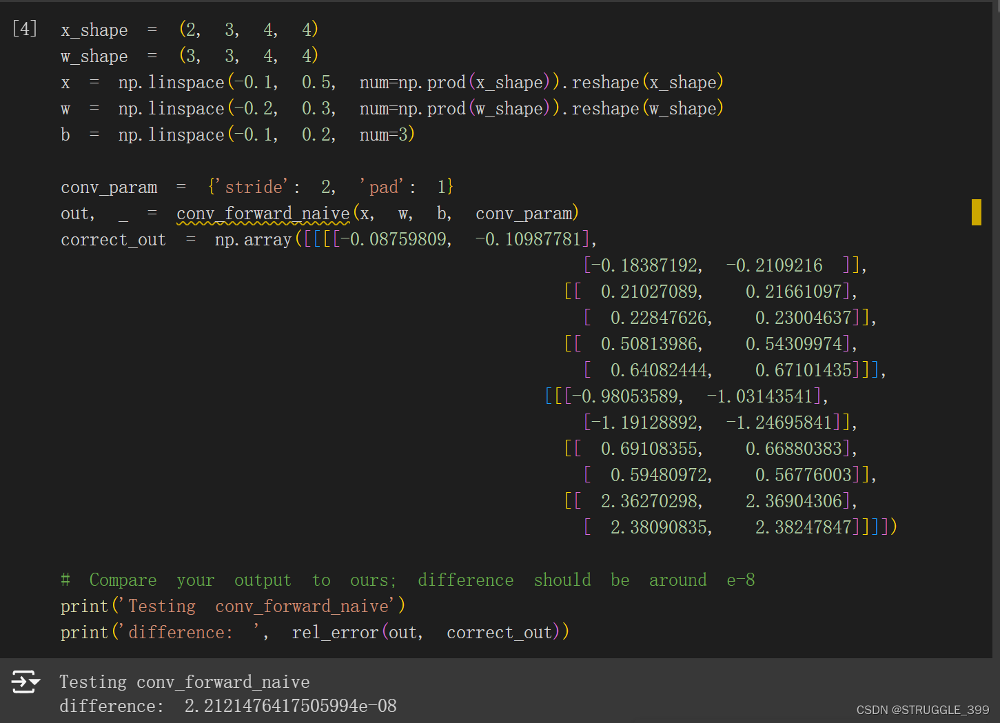
测试结果如下:
【优化】:这里实现的 conv_forward_naive 使用了四重 for 循环,是一个表示卷积操作比较清晰的代码,算是半向量化代码的实现,最少可以使用两重 for 循环实现卷积操作。
第一步,优化掉一重循环:
for n in range(N): # for each datapoint
    for i in range(H_out):
    	for j in range(W_out):
            # 获取当前卷积窗口
            window = x[n, :, i*stride:i*stride+HH, j*stride:j*stride+WW]
            out[n, :, i, j] = np.sum(w * window, axis=(1, 2, 3)) + b
第二步,优化最外层循环:
for i in range(H_out):
	for j in range(W_out):
        # 获取当前卷积窗口
        window = x[:, :, i*stride:i*stride+HH, j*stride:j*stride+WW]
        out[:, :, i, j] = np.sum(w.reshape((1, F, C, HH, WW)) * window.reshape(N, 1, C, HH, WW), axis=(2, 3, 4)) + b
优化后的代码,优化的方法主要就是利用广播机制,其结果是一样的。
【注意】作业中没有要求写出上面优化的代码,原始使用四重 for 循环的代码算是比较清晰的代码,直接用原始版本的代码也是ok的。
conv_backward_naive
根据卷积操作的公式,不难得到梯度的计算方法,具体代码如下:
def conv_backward_naive(dout, cache):
    """A naive implementation of the backward pass for a convolutional layer.

    Inputs:
    - dout: Upstream derivatives.
    - cache: A tuple of (x, w, b, conv_param) as in conv_forward_naive

    Returns a tuple of:
    - dx: Gradient with respect to x
    - dw: Gradient with respect to w
    - db: Gradient with respect to b
    """
    dx, dw, db = None, None, None
    ###########################################################################
    # TODO: Implement the convolutional backward pass.                        #
    ###########################################################################
    # *****START OF YOUR CODE (DO NOT DELETE/MODIFY THIS LINE)*****

    x, w, b, conv_param = cache
    dx, dw, db = np.zeros(x.shape), np.zeros(w.shape), np.zeros(b.shape)

    stride, pad = conv_param['stride'], conv_param['pad']
    N, C, H, W = x.shape
    F, C, HH, WW = w.shape
    N, F, H_out, W_out = dout.shape

    for n in range(N): # for each datapoint
        for k in range(F): # for each filter
            for i in range(H_out):
                for j in range(W_out):
                    dx[n, :, i*stride:i*stride+HH, j*stride:j*stride+WW] += w[k] * dout[n, k, i, j]
                    dw[k] += x[n, :, i*stride:i*stride+HH, j*stride:j*stride+WW] * dout[n, k, i, j]
                    db[k] += dout[n, k, i, j]

    # 消除原来x填充的边界
    dx = dx[:, :, pad:H-pad, pad:W-pad]
    # *****END OF YOUR CODE (DO NOT DELETE/MODIFY THIS LINE)*****
    ###########################################################################
    #                             END OF YOUR CODE                            #
    ###########################################################################
    return dx, dw, db
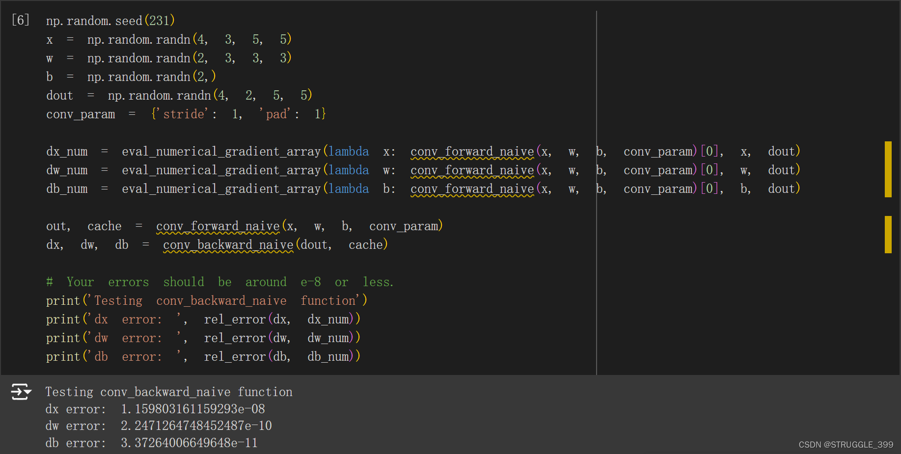
运行测试如下:
【优化】这里实现的 conv_backward_naive 使用了四重 for 循环,是一个表示卷积操作比较清晰的代码,算是半向量化代码的实现,最少可以使用两重 for 循环实现卷积操作。
第一步,优化掉一重循环:
for n in range(N):
    for i in range(H_out):
        for j in range(W_out):
            dx[n, :, i*stride:i*stride+HH, j*stride:j*stride+WW] += np.sum(w * dout[n, :, i, j].reshape((F, 1, 1, 1)), axis=0)
            dw += x[n, :, i*stride:i*stride+HH, j*stride:j*stride+WW].reshape((1, C, HH, WW)) * dout[n, :, i, j].reshape((F, 1, 1, 1))
            db += dout[n, :, i, j]
第二步,优化最外层循环:
for i in range(H_out):
    for j in range(W_out):
        dx[:, :, i*stride:i*stride+HH, j*stride:j*stride+WW] += np.sum(w.reshape((1, F, C, HH, WW)) * dout[:, :, i, j].reshape((N, F, 1, 1, 1)), axis=1)
        dw += np.sum(x[:, :, i*stride:i*stride+HH, j*stride:j*stride+WW].reshape((N, 1, C, HH, WW)) * dout[:, :, i, j].reshape((N, F, 1, 1, 1)), axis=0)
        db += np.sum(dout[:, :, i, j], axis=0)
优化后的代码,优化的方法主要就是利用广播机制,其结果是一样的。
【注意】作业中没有要求写出上面优化的代码,原始使用四重 for 循环的代码算是比较清晰的代码,直接用原始版本的代码也是ok的。
max_pool_forward_naive
max pool操作实现思路如下:
- 计算输出大小。
- 对于每个输入数据点,进行 max pool 操作。
- 首先获取池化窗口
window。 - 通过
np.max(window, axis=(1, 2))在其空间维度上求最大值。
- 首先获取池化窗口
def max_pool_forward_naive(x, pool_param):
    """A naive implementation of the forward pass for a max-pooling layer.

    Inputs:
    - x: Input data, of shape (N, C, H, W)
    - pool_param: dictionary with the following keys:
      - 'pool_height': The height of each pooling region
      - 'pool_width': The width of each pooling region
      - 'stride': The distance between adjacent pooling regions

    No padding is necessary here, eg you can assume:
      - (H - pool_height) % stride == 0
      - (W - pool_width) % stride == 0

    Returns a tuple of:
    - out: Output data, of shape (N, C, H', W') where H' and W' are given by
      H' = 1 + (H - pool_height) / stride
      W' = 1 + (W - pool_width) / stride
    - cache: (x, pool_param)
    """
    out = None
    ###########################################################################
    # TODO: Implement the max-pooling forward pass                            #
    ###########################################################################
    # *****START OF YOUR CODE (DO NOT DELETE/MODIFY THIS LINE)*****

    N, C, H, W = x.shape
    pool_height, pool_width, stride = pool_param['pool_height'], pool_param['pool_width'], pool_param['stride']

    H_out = 1 + (H - pool_height) / stride
    W_out = 1 + (W - pool_width) / stride

    out = np.zeros((N, C, H_out, W_out))

    for n in range(N):
        for i in range(H_out):
            for j in range(W_out):
                # 获取池化窗口
                window = x[n, :, i*stride:i*stride+pool_height, j*stride:j*stride+pool_width]
                out[n, :, i, j] = np.max(window, axis=(1, 2))

    # *****END OF YOUR CODE (DO NOT DELETE/MODIFY THIS LINE)*****
    ###########################################################################
    #                             END OF YOUR CODE                            #
    ###########################################################################
    cache = (x, pool_param)
    return out, cache
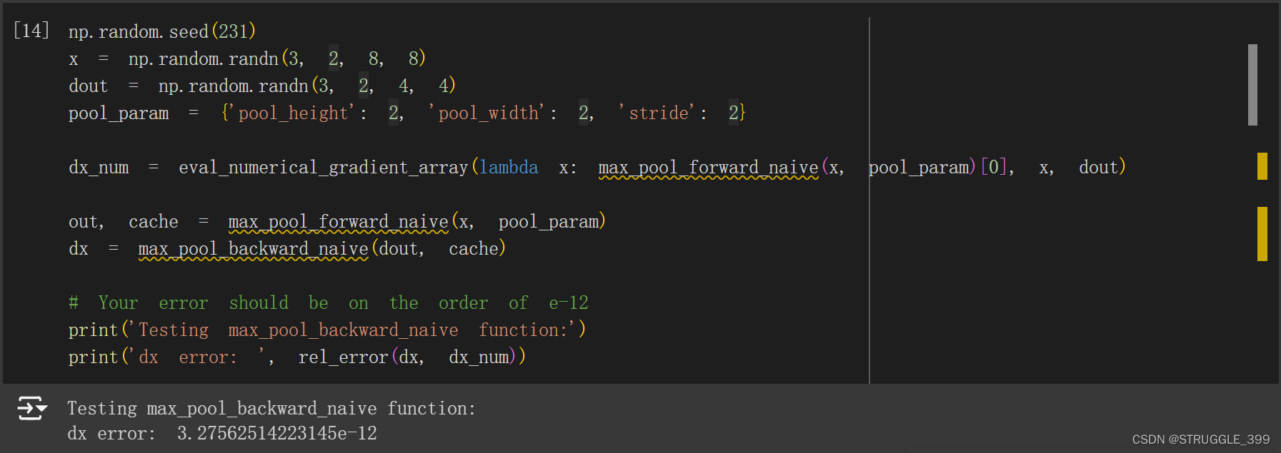
运行测试如下:

【优化】max_pool_forward_naive 可以再优化掉最外层循环,核心代码如下:
for i in range(H_out):
    for j in range(W_out):
        window = x[:, :, i*stride:i*stride+pool_height, j*stride:j*stride+pool_width]
        out[:, :, i, j] = np.max(window, axis=(2, 3))
max_pool_backward_naive
max pool 的反向传播代码有点类似于 ReLU 激活函数的反向传播代码,实现思路是:
- 首先获取池化窗口
window。 - 通过
np.argmax(window)获取max_index,再通过np.unravel_index(max_index, window.shape)获取其在window中的位置row, col。 - 在池化窗口对应的最大值
(row, col)位置的梯度就是dout[n, c, i, j],在此窗口内的其他元素的梯度均为 0。
def max_pool_backward_naive(dout, cache):
    """A naive implementation of the backward pass for a max-pooling layer.

    Inputs:
    - dout: Upstream derivatives
    - cache: A tuple of (x, pool_param) as in the forward pass.

    Returns:
    - dx: Gradient with respect to x
    """
    dx = None
    ###########################################################################
    # TODO: Implement the max-pooling backward pass                           #
    ###########################################################################
    # *****START OF YOUR CODE (DO NOT DELETE/MODIFY THIS LINE)*****

    x, pool_param = cache
    N, C, H, W = x.shape
    dx = np.zeros(x.shape)

    pool_height, pool_width, stride = pool_param['pool_height'], pool_param['pool_width'], pool_param['stride']

    H_out = 1 + (H - pool_height) // stride
    W_out = 1 + (W - pool_width) // stride

    for n in range(N):
      for c in range(C):
        for i in range(H_out):
          for j in range(W_out):
            window = x[n, c, i*stride:i*stride+pool_height, j*stride:j*stride+pool_width]
            max_index = np.argmax(window)
            row, col = np.unravel_index(max_index, window.shape)
            dx[n, c, i*stride+row, j*stride+col] += dout[n, c, i, j]
    # *****END OF YOUR CODE (DO NOT DELETE/MODIFY THIS LINE)*****
    ###########################################################################
    #                             END OF YOUR CODE                            #
    ###########################################################################
    return dx
测试结果如下:
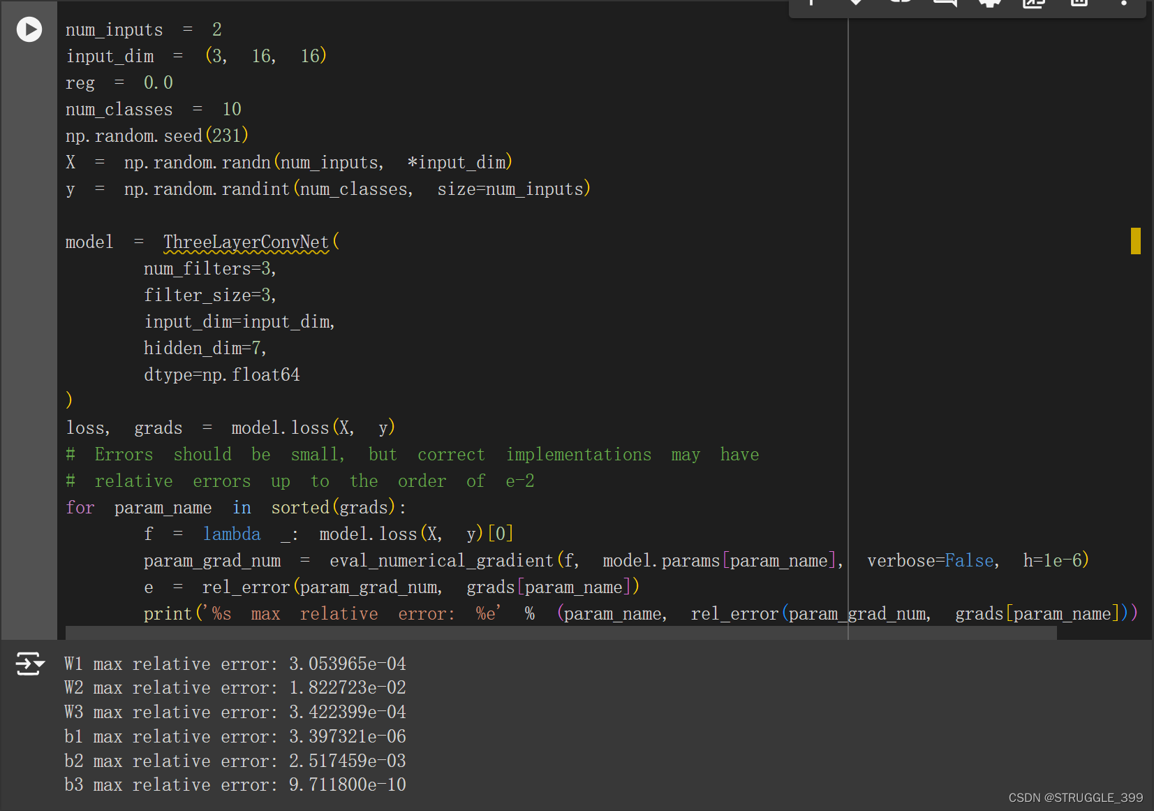
Three-Layer Convolutional Network
init
init 方法用于初始化三层神经网络,三层卷积神经网络的结构如下:
conv - relu - 2x2 max pool - affine - relu - affine - softmax
代码如下:
def __init__(
    self,
    input_dim=(3, 32, 32),
    num_filters=32,
    filter_size=7,
    hidden_dim=100,
    num_classes=10,
    weight_scale=1e-3,
    reg=0.0,
    dtype=np.float32,
):
    """
    Initialize a new network.

    Inputs:
    - input_dim: Tuple (C, H, W) giving size of input data
    - num_filters: Number of filters to use in the convolutional layer
    - filter_size: Width/height of filters to use in the convolutional layer
    - hidden_dim: Number of units to use in the fully-connected hidden layer
    - num_classes: Number of scores to produce from the final affine layer.
    - weight_scale: Scalar giving standard deviation for random initialization
      of weights.
    - reg: Scalar giving L2 regularization strength
    - dtype: numpy datatype to use for computation.
    """
    self.params = {}
    self.reg = reg
    self.dtype = dtype

    ############################################################################
    # TODO: Initialize weights and biases for the three-layer convolutional    #
    # network. Weights should be initialized from a Gaussian centered at 0.0   #
    # with standard deviation equal to weight_scale; biases should be          #
    # initialized to zero. All weights and biases should be stored in the      #
    #  dictionary self.params. Store weights and biases for the convolutional  #
    # layer using the keys 'W1' and 'b1'; use keys 'W2' and 'b2' for the       #
    # weights and biases of the hidden affine layer, and keys 'W3' and 'b3'    #
    # for the weights and biases of the output affine layer.                   #
    #                                                                          #
    # IMPORTANT: For this assignment, you can assume that the padding          #
    # and stride of the first convolutional layer are chosen so that           #
    # **the width and height of the input are preserved**. Take a look at      #
    # the start of the loss() function to see how that happens.                #
    ############################################################################
    # *****START OF YOUR CODE (DO NOT DELETE/MODIFY THIS LINE)*****

    C, H, W = input_dim
    self.params['W1'] = np.random.randn(num_filters, C, filter_size, filter_size) * weight_scale
    self.params['b1'] = np.zeros(num_filters)

    # 经过 2x2 max pool 后大小缩减为原来的四分之一
    self.params['W2'] = np.random.randn(num_filters * H * W // 4, hidden_dim) * weight_scale
    self.params['b2'] = np.zeros(hidden_dim)

    self.params['W3'] = np.random.randn(hidden_dim, num_classes) * weight_scale
    self.params['b3'] = np.zeros(num_classes)

    # *****END OF YOUR CODE (DO NOT DELETE/MODIFY THIS LINE)*****
    ############################################################################
    #                             END OF YOUR CODE                             #
    ############################################################################

    for k, v in self.params.items():
		self.params[k] = v.astype(dtype)
loss
cs231n/layer_utils.py 提供了许多 “Sanwidch Layer”,包括 conv - relu - maxpool、conv - relu、affine - relu 等等结构的前向传递和后向传递函数,直接使用即可。代码如下:
def loss(self, X, y=None):
    """
    Evaluate loss and gradient for the three-layer convolutional network.

    Input / output: Same API as TwoLayerNet in fc_net.py.
    """
    W1, b1 = self.params["W1"], self.params["b1"]
    W2, b2 = self.params["W2"], self.params["b2"]
    W3, b3 = self.params["W3"], self.params["b3"]

    # pass conv_param to the forward pass for the convolutional layer
    # Padding and stride chosen to preserve the input spatial size
    filter_size = W1.shape[2]
    conv_param = {"stride": 1, "pad": (filter_size - 1) // 2}

    # pass pool_param to the forward pass for the max-pooling layer
    pool_param = {"pool_height": 2, "pool_width": 2, "stride": 2}

    scores = None
    ############################################################################
    # TODO: Implement the forward pass for the three-layer convolutional net,  #
    # computing the class scores for X and storing them in the scores          #
    # variable.                                                                #
    #                                                                          #
    # Remember you can use the functions defined in cs231n/fast_layers.py and  #
    # cs231n/layer_utils.py in your implementation (already imported).         #
    ############################################################################
    # *****START OF YOUR CODE (DO NOT DELETE/MODIFY THIS LINE)*****

    a, cache1 = conv_relu_pool_forward(X, W1, b1, conv_param, pool_param)
    a, cache2 = affine_relu_forward(a, W2, b2)
    scores, cache3 = affine_forward(a, W3, b3)

    # *****END OF YOUR CODE (DO NOT DELETE/MODIFY THIS LINE)*****
    ############################################################################
    #                             END OF YOUR CODE                             #
    ############################################################################

    if y is None:
        return scores

    loss, grads = 0, {}
    ############################################################################
    # TODO: Implement the backward pass for the three-layer convolutional net, #
    # storing the loss and gradients in the loss and grads variables. Compute  #
    # data loss using softmax, and make sure that grads[k] holds the gradients #
    # for self.params[k]. Don't forget to add L2 regularization!               #
    #                                                                          #
    # NOTE: To ensure that your implementation matches ours and you pass the   #
    # automated tests, make sure that your L2 regularization includes a factor #
    # of 0.5 to simplify the expression for the gradient.                      #
    ############################################################################
    # *****START OF YOUR CODE (DO NOT DELETE/MODIFY THIS LINE)*****

    # 计算 softmax loss 和 dscores
    loss, dscores = softmax_loss(scores, y)
    # 加上 L2 正则化损失
    loss += 0.5 * self.reg * (np.sum(W1 * W1) + np.sum(W2 * W2) + np.sum(W3 * W3))

    # 反向传播
    dx, dw3, db3 = affine_backward(dscores, cache3)
    dx, dw2, db2 = affine_relu_backward(dx, cache2)
    dx, dw1, db1 = conv_relu_pool_backward(dx, cache1)

    grads['W1'], grads['b1'] = dw1 + self.reg * W1, db1
    grads['W2'], grads['b2'] = dw2 + self.reg * W2, db2
    grads['W3'], grads['b3'] = dw3 + self.reg * W3, db3

    # *****END OF YOUR CODE (DO NOT DELETE/MODIFY THIS LINE)*****
    ############################################################################
    #                             END OF YOUR CODE                             #
    ############################################################################

    return loss, grads
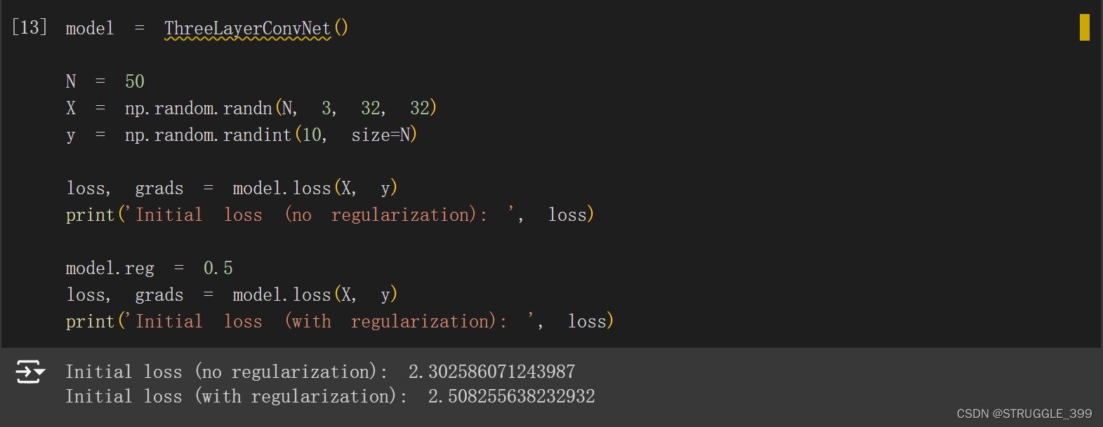
测试如下:
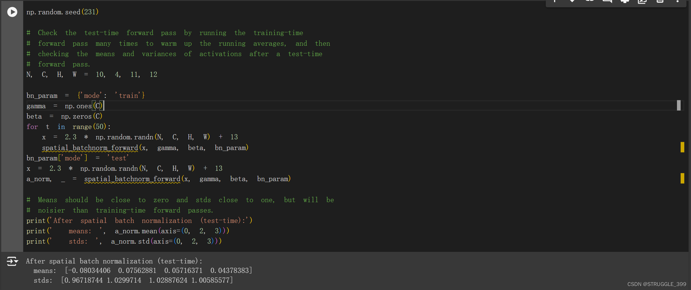
Spatial Batch Normalization
spatial batch normalization 可以使用 batch normalization 进行实现。
spatial_batchnorm_forward
spatial_batchnorm_forward 的实现思路为:
- 将 x 的第二个轴移动到最后,最终形状为
(NxHxW, C)。 - 调用
batchnorm_forward。 batchnorm_forward的输出重塑为四维数组,并将最后一个轴移动到第二个轴。
def spatial_batchnorm_forward(x, gamma, beta, bn_param):
    """Computes the forward pass for spatial batch normalization.

    Inputs:
    - x: Input data of shape (N, C, H, W)
    - gamma: Scale parameter, of shape (C,)
    - beta: Shift parameter, of shape (C,)
    - bn_param: Dictionary with the following keys:
      - mode: 'train' or 'test'; required
      - eps: Constant for numeric stability
      - momentum: Constant for running mean / variance. momentum=0 means that
        old information is discarded completely at every time step, while
        momentum=1 means that new information is never incorporated. The
        default of momentum=0.9 should work well in most situations.
      - running_mean: Array of shape (D,) giving running mean of features
      - running_var Array of shape (D,) giving running variance of features

    Returns a tuple of:
    - out: Output data, of shape (N, C, H, W)
    - cache: Values needed for the backward pass
    """

    out, cache = None, None

    ###########################################################################
    # TODO: Implement the forward pass for spatial batch normalization.       #
    #                                                                         #
    # HINT: You can implement spatial batch normalization by calling the      #
    # vanilla version of batch normalization you implemented above.           #
    # Your implementation should be very short; ours is less than five lines. #
    ###########################################################################
    # *****START OF YOUR CODE (DO NOT DELETE/MODIFY THIS LINE)*****

    N, C, H, W = x.shape
    x = np.moveaxis(x, 1, -1).reshape(-1, C) # of shape (NxHxW, C)
    out, cache = batchnorm_forward(x, gamma, beta, bn_param)
    out = np.moveaxis(out.reshape(N, H, W, C), -1, 1)

    # *****END OF YOUR CODE (DO NOT DELETE/MODIFY THIS LINE)*****
    ###########################################################################
    #                             END OF YOUR CODE                            #
    ###########################################################################

    return out, cache

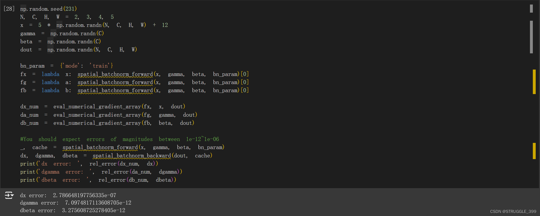
spatial_batchnorm_backward
spatial_batchnorm_backward 的实现思路与 spatial_batchnorm_forward 是一样的,区别在于调用 batchnorm_backward。
def spatial_batchnorm_backward(dout, cache):
    """Computes the backward pass for spatial batch normalization.

    Inputs:
    - dout: Upstream derivatives, of shape (N, C, H, W)
    - cache: Values from the forward pass

    Returns a tuple of:
    - dx: Gradient with respect to inputs, of shape (N, C, H, W)
    - dgamma: Gradient with respect to scale parameter, of shape (C,)
    - dbeta: Gradient with respect to shift parameter, of shape (C,)
    """
    dx, dgamma, dbeta = None, None, None

    ###########################################################################
    # TODO: Implement the backward pass for spatial batch normalization.      #
    #                                                                         #
    # HINT: You can implement spatial batch normalization by calling the      #
    # vanilla version of batch normalization you implemented above.           #
    # Your implementation should be very short; ours is less than five lines. #
    ###########################################################################
    # *****START OF YOUR CODE (DO NOT DELETE/MODIFY THIS LINE)*****

    N, C, H, W = dout.shape
    dout = np.moveaxis(dout, 1, -1).reshape(-1, C)
    dx, dgamma, dbeta = batchnorm_backward(dout, cache)
    dx = np.moveaxis(dx.reshape(N, H, W, C), -1, 1)

    # *****END OF YOUR CODE (DO NOT DELETE/MODIFY THIS LINE)*****
    ###########################################################################
    #                             END OF YOUR CODE                            #
    ###########################################################################

    return dx, dgamma, dbeta
Spatial Layer Normalization
Spatial Layer Normalization 不是作业中的要求,这里给出 spatial_layernorm_forward 和 spatial_layernorm_backward 的实现,为了更好地过渡到 Spatial Group Normalization,因为 Spatial Group Normalization 和 Spatial Layer Normalization 是很类似的。
spatial_layernorm_forward
def spatial_layernorm_forward(x, gamma, beta, ln_param):
    """Forward pass for spatial layer normalization.

    During both training and test-time, the incoming data is normalized per data-point,
    before being scaled by gamma and beta parameters identical to that of batch normalization.

    Note that in contrast to batch normalization, the behavior during train and test-time for
    spatial layer normalization are identical, and we do not need to keep track of running averages
    of any sort.

    Input:
    - x: Data of shape (N, C, H, W)
    - gamma: Scale parameter of shape (1, C, 1, 1)
    - beta: Shift paremeter of shape (1, C, 1, 1)
    - ln_param: Dictionary with the following keys:
        - eps: Constant for numeric stability

    Returns a tuple of:
    - out: of shape (N, C, H, W)
    - cache: A tuple of values needed in the backward pass
    """
    out, cache = None, None
    eps = ln_param.get("eps", 1e-5)
    ###########################################################################
    # TODO: Implement the training-time forward pass for layer norm.          #
    # Normalize the incoming data, and scale and  shift the normalized data   #
    #  using gamma and beta.                                                  #
    # HINT: this can be done by slightly modifying your training-time         #
    # implementation of  batch normalization, and inserting a line or two of  #
    # well-placed code. In particular, can you think of any matrix            #
    # transformations you could perform, that would enable you to copy over   #
    # the batch norm code and leave it almost unchanged?                      #
    ###########################################################################
    # *****START OF YOUR CODE (DO NOT DELETE/MODIFY THIS LINE)*****

    N, C, H, W = x.shape
    x_mean = np.mean(x, aixs=(1, 2, 3), keepdims=True)
    x_var = np.var(x, axis=(1, 2, 3), keepdims=True)
    x_norm = (x - x_mean) / np.sqrt(x_var + eps)

    out = gamma * x_norm + beta

    cache = (x, x_mean, x_var, x_norm, gamma, beta, eps)

    # *****END OF YOUR CODE (DO NOT DELETE/MODIFY THIS LINE)*****
    ###########################################################################
    #                             END OF YOUR CODE                            #
    ###########################################################################
    return out, cache
spatial_layernorm_backward
def spatial_layernorm_backward(dout, cache):
    """Backward pass for spatial layer normalization.

    For this implementation, you can heavily rely on the work you've done already
    for batch normalization.

    Inputs:
    - dout: Upstream derivatives, of shape (N, C, H, W)
    - cache: Variable of intermediates from layernorm_forward.

    Returns a tuple of:
    - dx: Gradient with respect to inputs x, of shape (N, C, H, W)
    - dgamma: Gradient with respect to scale parameter gamma, of shape (1, C, 1, 1)
    - dbeta: Gradient with respect to shift parameter beta, of shape (1, C, 1, 1)
    """
    dx, dgamma, dbeta = None, None, None
    ###########################################################################
    # TODO: Implement the backward pass for layer norm.                       #
    #                                                                         #
    # HINT: this can be done by slightly modifying your training-time         #
    # implementation of batch normalization. The hints to the forward pass    #
    # still apply!                                                            #
    ###########################################################################
    # *****START OF YOUR CODE (DO NOT DELETE/MODIFY THIS LINE)*****

    x, x_mean, x_var, x_norm, gamma, beta, eps = cache
    N, C, H, W = x.shape
    D = C * H * W

    dx_norm = gamma * dout
    dgamma = np.sum(dout * x_norm, axis=(0, 2, 3), keepdims=True)
    dbeta = np.sum(dout, axis=(0, 2, 3), keepdims=True)

    dx_var = np.sum(-0.5 * dx_norm * x_norm / (x_var + eps), axis=(1, 2, 3), keepdims=True)
    dx_mean = np.sum(-dx_norm / np.sqrt(x_var + eps), axis=(1, 2, 3), keepdims=True)

    dx = dx_norm / np.sqrt(x_var + eps) + 2 / D * dx_var * (x - x_mean) + dx_mean / D

    # *****END OF YOUR CODE (DO NOT DELETE/MODIFY THIS LINE)*****
    ###########################################################################
    #                             END OF YOUR CODE                            #
    ###########################################################################
    return dx, dgamma, dbeta
Spatial Group Normalization
Group Normalization 与 Batch Normalization、Layer Normalization 的区别如下图所示:
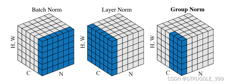
在论文中,给出了 group normalization 的 TensorFlow 实现,对应的 numpy 实现是类似的。
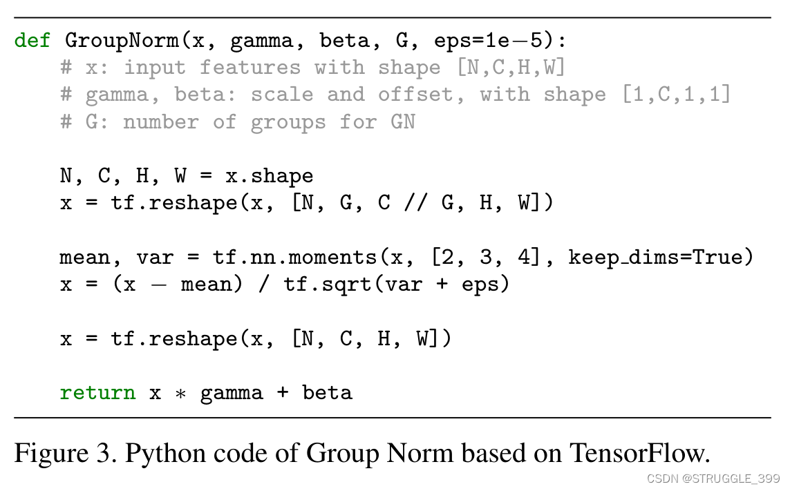
Group Normalization 其实与 Layer Normalization 是比较相似的。
spatial_groupnorm_forward
我们可以仿照论文中给出的 GN 实现代码,实现思路为:
- 将
xreshape 成 5 维数组(将通道分成 C 组)。 - 求
x最后三个维度的均值和方差,注意需要keepdims=True参数,因为在归一化时才能正常应用广播机制,不然需要reshape成 5 维数组,形状为(N, G, 1, 1, 1)。 - 归一化操作。
- 计算输出。
def spatial_groupnorm_forward(x, gamma, beta, G, gn_param):
    """Computes the forward pass for spatial group normalization.

    In contrast to layer normalization, group normalization splits each entry in the data into G
    contiguous pieces, which it then normalizes independently. Per-feature shifting and scaling
    are then applied to the data, in a manner identical to that of batch normalization and layer
    normalization.

    Inputs:
    - x: Input data of shape (N, C, H, W)
    - gamma: Scale parameter, of shape (1, C, 1, 1)
    - beta: Shift parameter, of shape (1, C, 1, 1)
    - G: Integer mumber of groups to split into, should be a divisor of C
    - gn_param: Dictionary with the following keys:
      - eps: Constant for numeric stability

    Returns a tuple of:
    - out: Output data, of shape (N, C, H, W)
    - cache: Values needed for the backward pass
    """
    out, cache = None, None
    eps = gn_param.get("eps", 1e-5)
    ###########################################################################
    # TODO: Implement the forward pass for spatial group normalization.       #
    # This will be extremely similar to the layer norm implementation.        #
    # In particular, think about how you could transform the matrix so that   #
    # the bulk of the code is similar to both train-time batch normalization  #
    # and layer normalization!                                                #
    ###########################################################################
    # *****START OF YOUR CODE (DO NOT DELETE/MODIFY THIS LINE)*****

    N, C, H, W = x.shape
    x = x.reshape(N, G, C // G, H, W)

    x_mean = np.mean(x, axis=(2, 3, 4), keepdims=True)
    x_var = np.var(x, axis=(2, 3, 4), keepdims=True)

    x_norm = (x - x_mean) / np.sqrt(x_var + eps)
    x_norm = x_norm.reshape(N, C, H, W)
    out = gamma * x_norm + beta

    cache = (x, x_norm, x_mean, x_var, gamma, beta, G, eps)

    # *****END OF YOUR CODE (DO NOT DELETE/MODIFY THIS LINE)*****
    ###########################################################################
    #                             END OF YOUR CODE                            #
    ###########################################################################
    return out, cache
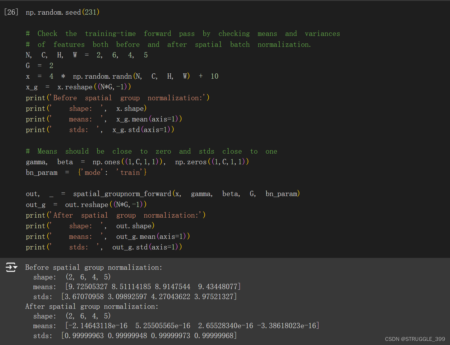
测试结果如下:
spatial_groupnorm_backward
Group Normalization 的实现与 Layer Normalization 的实现是相似的,因此我们可以仿照 Spatial Layer Normalization 的反向传播代码,只需要做一些调整即可。
def spatial_groupnorm_backward(dout, cache):
    """Computes the backward pass for spatial group normalization.

    Inputs:
    - dout: Upstream derivatives, of shape (N, C, H, W)
    - cache: Values from the forward pass

    Returns a tuple of:
    - dx: Gradient with respect to inputs, of shape (N, C, H, W)
    - dgamma: Gradient with respect to scale parameter, of shape (1, C, 1, 1)
    - dbeta: Gradient with respect to shift parameter, of shape (1, C, 1, 1)
    """
    dx, dgamma, dbeta = None, None, None

    ###########################################################################
    # TODO: Implement the backward pass for spatial group normalization.      #
    # This will be extremely similar to the layer norm implementation.        #
    ###########################################################################
    # *****START OF YOUR CODE (DO NOT DELETE/MODIFY THIS LINE)*****

    x, x_norm, x_mean, x_var, gamma, beta, G, eps = cache
    N, C, H, W = dout.shape
	D = C // G * H * W

    dgamma = np.sum(dout * x_norm, axis=(0, 2, 3), keepdims=True)
    dbeta = np.sum(dout, axis=(0, 2, 3), keepdims=True)
    dx_norm = (dout * gamma).reshape(N, G, C // G, H, W)

    x_norm = x_norm.reshape(N, G, C // G, H, W)
    dx_var = np.sum(-0.5 * dx_norm * x_norm / (x_var + eps), axis=(2, 3, 4), keepdims=True)
    dx_mean = np.sum(-dx_norm / np.sqrt(x_var + eps), axis=(2, 3, 4), keepdims=True)
    dx = dx_norm / np.sqrt(x_var + eps) + 2 / D * dx_var * (x - x_mean) + dx_mean / D
    dx = dx.reshape(N, C, H, W)

    # *****END OF YOUR CODE (DO NOT DELETE/MODIFY THIS LINE)*****
    ###########################################################################
    #                             END OF YOUR CODE                            #
    ###########################################################################
    return dx, dgamma, dbeta
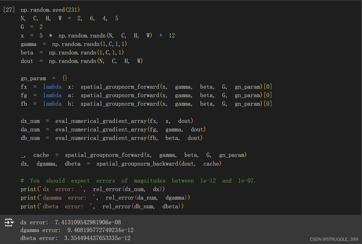
测试结果如下:
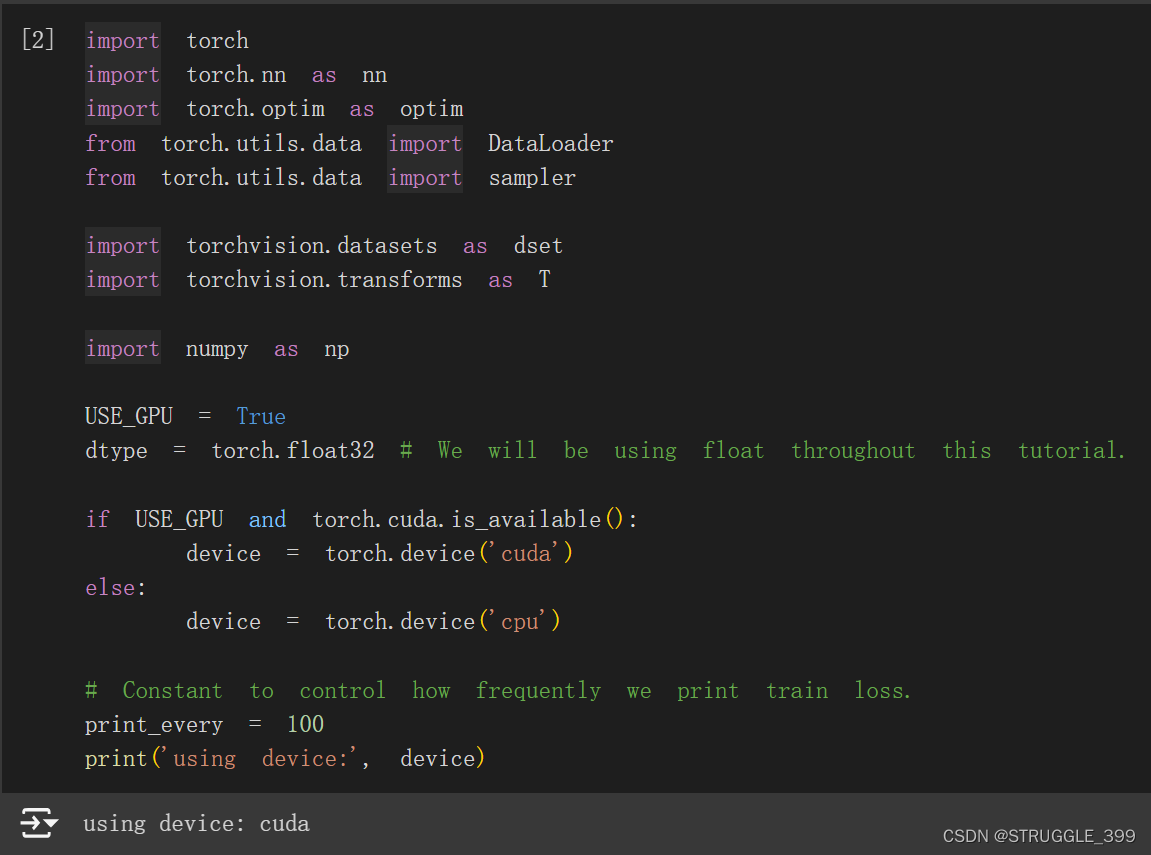
Q5: PyTorch on CIFAR-10
本作业有 5 个部分。 您将在三个不同的抽象级别上学习 PyTorch,
- 第一部分,准备:我们将使用 CIFAR-10 数据集。
- 第二部分,Barebones PyTorch:抽象级别 1,我们将直接使用最低级别的 PyTorch 张量(
Tensor)。 - 第三部分,PyTorch 模块 API:抽象级别 2,我们将使用
nn.Module定义任意神经网络架构。 - 第四部分,PyTorch Sequential API:抽象级别 3,我们将使用
nn.Sequential非常方便地定义线性前馈网络。 - 第五部分,CIFAR-10 开放式挑战:请实现您自己的网络,以在 CIFAR-10 上获得尽可能高的准确性。 您可以尝试任何层、优化器、超参数或其他高级功能。
| API | 灵活性 | 便捷性 |
|---|---|---|
| Barebone | 高 | 低 |
nn.Module | 高 | 中 |
nn.Sequential | 低 | 高 |
在完成这个作业时,需要使用 GPU 加速,我们需要在 Google Colab 上调整使用的硬件为 GPU。
Barebone PyTorch
首先定义一个 flatten 函数(作业中已给出,不需要实现):
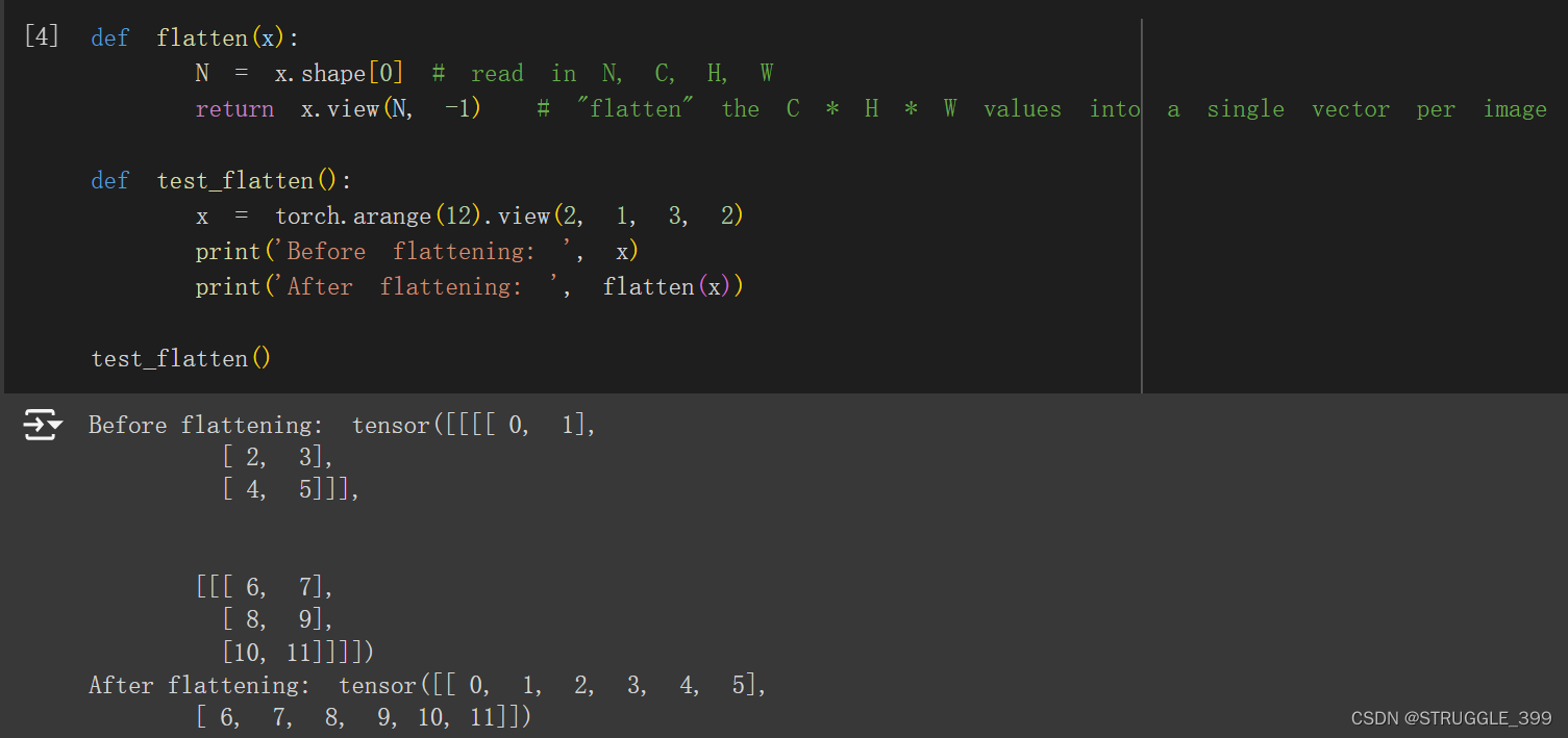
view 函数类似于 numpy 中的 reshape 函数。下面是一个两层全连接神经网络的例子(作业中已给出):
Two-Layer Network
import torch.nn.functional as F  # useful stateless functions

def two_layer_fc(x, params):
    """
    A fully-connected neural networks; the architecture is:
    NN is fully connected -> ReLU -> fully connected layer.
    Note that this function only defines the forward pass;
    PyTorch will take care of the backward pass for us.

    The input to the network will be a minibatch of data, of shape
    (N, d1, ..., dM) where d1 * ... * dM = D. The hidden layer will have H units,
    and the output layer will produce scores for C classes.

    Inputs:
    - x: A PyTorch Tensor of shape (N, d1, ..., dM) giving a minibatch of
      input data.
    - params: A list [w1, w2] of PyTorch Tensors giving weights for the network;
      w1 has shape (D, H) and w2 has shape (H, C).

    Returns:
    - scores: A PyTorch Tensor of shape (N, C) giving classification scores for
      the input data x.
    """
    # first we flatten the image
    x = flatten(x)  # shape: [batch_size, C x H x W]

    w1, w2 = params

    # Forward pass: compute predicted y using operations on Tensors. Since w1 and
    # w2 have requires_grad=True, operations involving these Tensors will cause
    # PyTorch to build a computational graph, allowing automatic computation of
    # gradients. Since we are no longer implementing the backward pass by hand we
    # don't need to keep references to intermediate values.
    # you can also use `.clamp(min=0)`, equivalent to F.relu()
    x = F.relu(x.mm(w1))
    x = x.mm(w2)
    return x


def two_layer_fc_test():
    hidden_layer_size = 42
    x = torch.zeros((64, 50), dtype=dtype)  # minibatch size 64, feature dimension 50
    w1 = torch.zeros((50, hidden_layer_size), dtype=dtype)
    w2 = torch.zeros((hidden_layer_size, 10), dtype=dtype)
    scores = two_layer_fc(x, [w1, w2])
    print(scores.size())  # you should see [64, 10]

two_layer_fc_test() # torch.Size([64, 10])
Three-Layer ConvNet
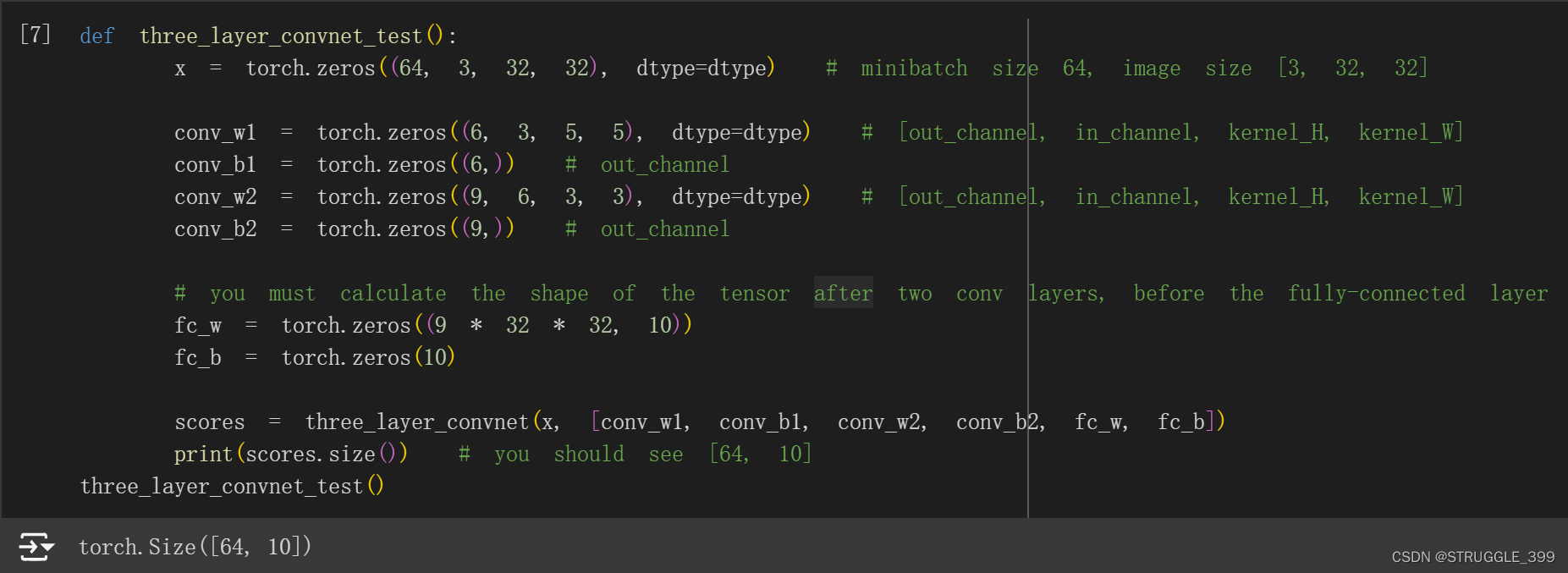
在这里,您将完成函数 Three_layer_convnet 的实现,该函数将执行三层卷积网络的前向传递。 像上面一样,我们可以通过网络传递零来立即测试我们的实现。 网络应具有以下架构:
- 一个具有
channel_1个卷积核的卷积层(有偏移项),形状为:KW1xKH1,2 个零填充。 - ReLU 非线性。
- 一个具有
channel_2个卷积核的卷积层(有偏移项),形状为:KW2xKH2,1 个零填充。 - ReLU 非线性。
- 全连接层,产生 C 个类别的得分。
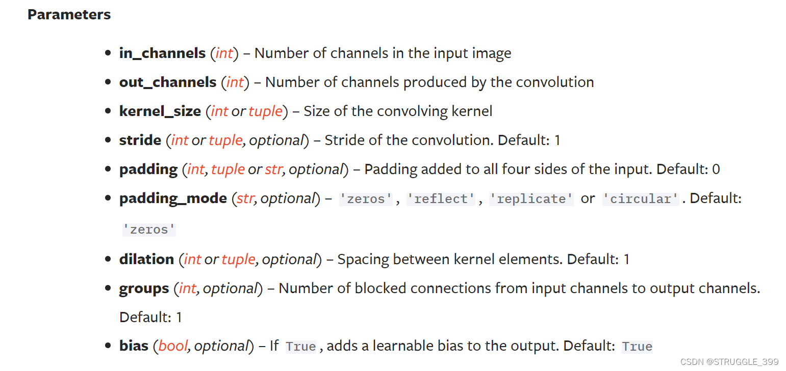
提示:对于卷积操作,可参考 Conv2d。注意卷积核的形状。
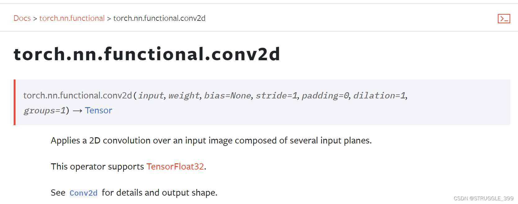

根据 PyTorch 文档,调用 torch.nn.functional.conv2d 函数至少需要传递 2 个参数,分别为输入(x, feature map tensor),所有卷积核的权重(weights),由于卷积层有偏移项,因此需要传递 bias 参数,以及 zero padding 的宽度。
根据以下公式可计算出卷积后输出的特征图的大小:
$$
\begin{aligned}
W^\prime &= (W-F+2P)/S+1\
H^\prime &= (H-F+2P)/S+1
\end{aligned}
$$
经过第一个卷积层和第二个卷积层后,空间维度大小不变,形状则分别为:(N, channel_1, H, W)、(N, channel_2, H, W)。
def three_layer_convnet(x, params):
    """
    Performs the forward pass of a three-layer convolutional network with the
    architecture defined above.

    Inputs:
    - x: A PyTorch Tensor of shape (N, 3, H, W) giving a minibatch of images
    - params: A list of PyTorch Tensors giving the weights and biases for the
      network; should contain the following:
      - conv_w1: PyTorch Tensor of shape (channel_1, 3, KH1, KW1) giving weights
        for the first convolutional layer
      - conv_b1: PyTorch Tensor of shape (channel_1,) giving biases for the first
        convolutional layer
      - conv_w2: PyTorch Tensor of shape (channel_2, channel_1, KH2, KW2) giving
        weights for the second convolutional layer
      - conv_b2: PyTorch Tensor of shape (channel_2,) giving biases for the second
        convolutional layer
      - fc_w: PyTorch Tensor giving weights for the fully-connected layer. Can you
        figure out what the shape should be?
      - fc_b: PyTorch Tensor giving biases for the fully-connected layer. Can you
        figure out what the shape should be?

    Returns:
    - scores: PyTorch Tensor of shape (N, C) giving classification scores for x
    """
    conv_w1, conv_b1, conv_w2, conv_b2, fc_w, fc_b = params
    scores = None
    ################################################################################
    # TODO: Implement the forward pass for the three-layer ConvNet.                #
    ################################################################################
    # *****START OF YOUR CODE (DO NOT DELETE/MODIFY THIS LINE)*****

    x = F.conv2d(x, conv_w1, bias=conv_b1, padding=2)
    x = F.relu(x)
    x = F.conv2d(x, conv_w2, bias=conv_b2, padding=1)
    x = F.relu(x)
    x = flatten(x)
    scores = x.mm(fc_w) + fc_b
    # *****END OF YOUR CODE (DO NOT DELETE/MODIFY THIS LINE)*****
    ################################################################################
    #                                 END OF YOUR CODE                             #
    ################################################################################
    return scores
测试如下:
Initialization
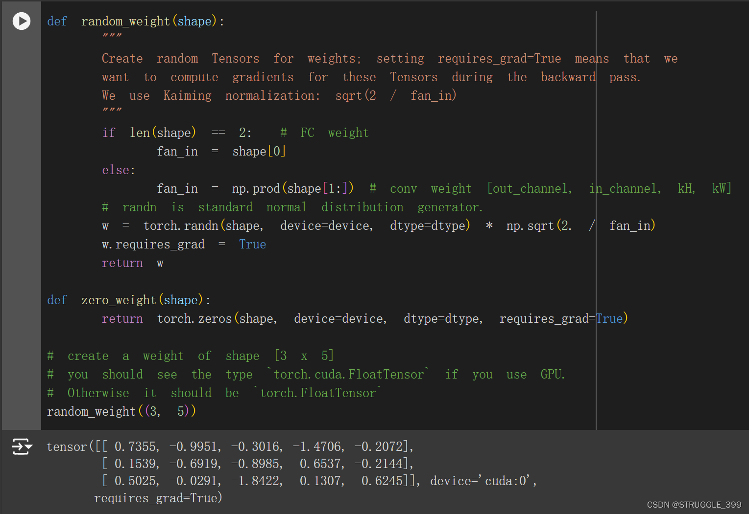
让我们编写几个实用方法(作业中已给出)来初始化模型的权重矩阵。
random_weight(shape),使用 Kaiming 归一化方法初始化权重张量。zero_weight(shape),用全零初始化权重张量。 对于实例化偏置参数很有用。
random_weight 函数使用 Kaiming 归一化初始化方法,在论文 He et al, Delving Deep into Rectifiers: Surpassing Human-Level Performance on ImageNet Classification 中描述。
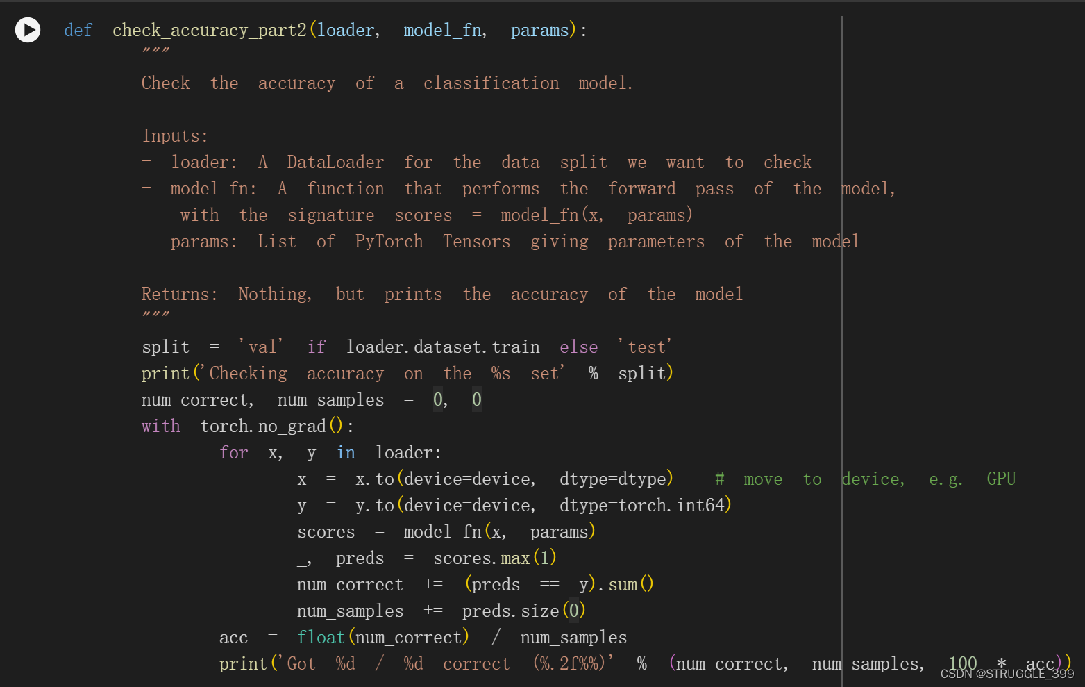
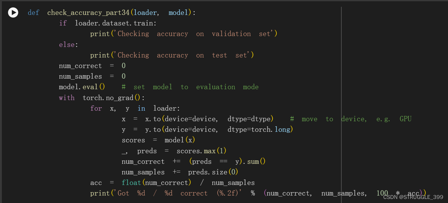
Check Accuracy
在训练模型时,我们将使用以下函数来检查我们的模型在训练集或验证集上的精度。在检查精度时,我们不需要计算任何梯度;因此,当我们计算得分时,我们不需要 PyTorch 来为我们构建计算图。为了防止生成计算图,我们在 torch.no_grad() 上下文管理器(Context Manager)下确定计算范围。
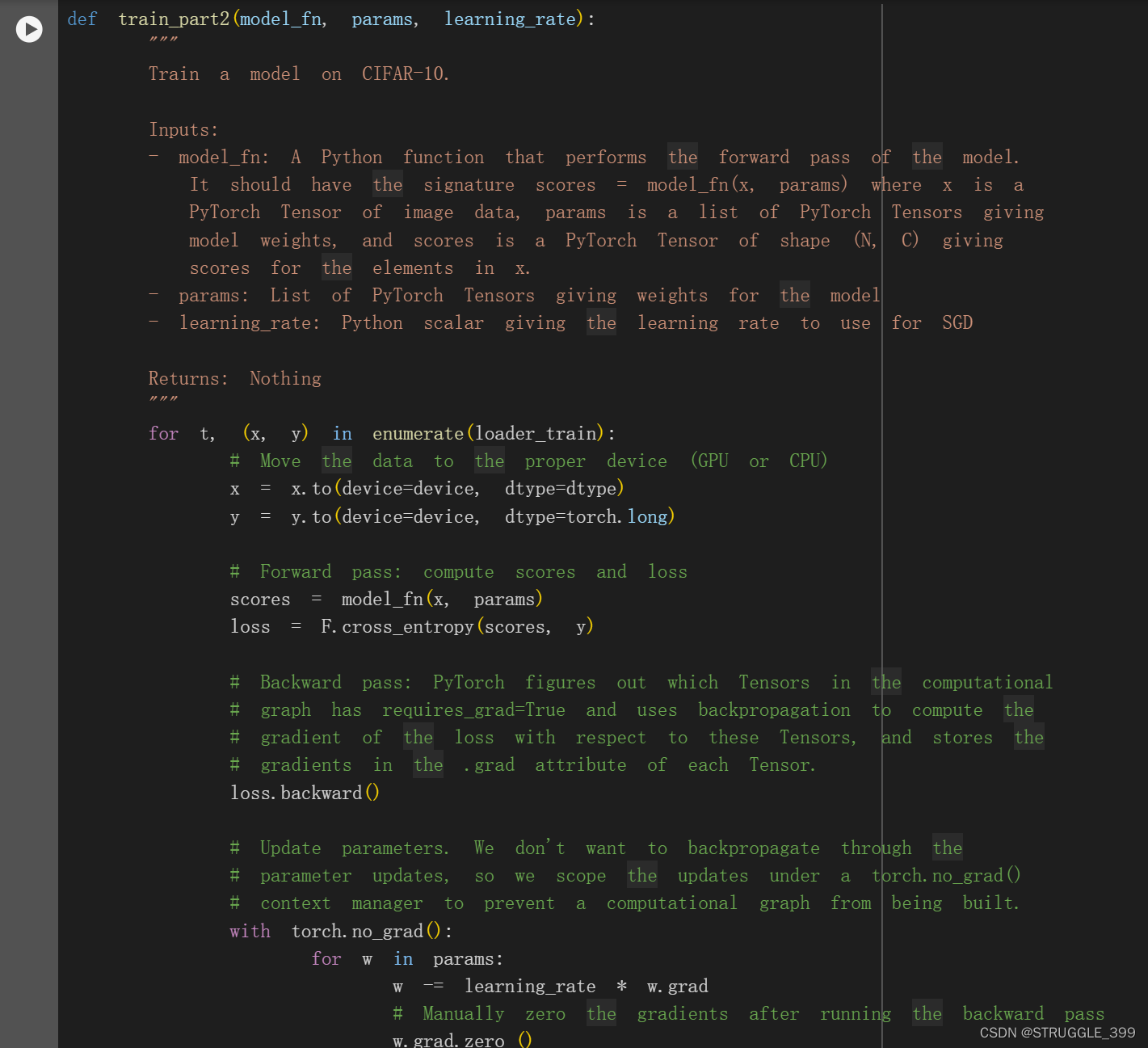
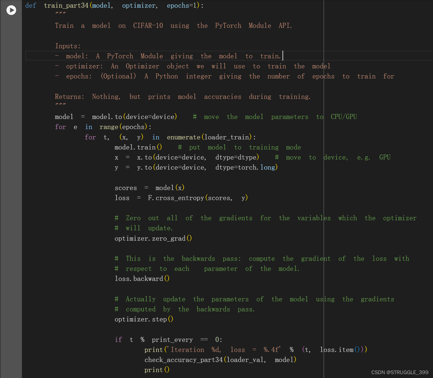
Traing Loop
我们现在可以建立一个基本的训练循环来训练我们的网络。 我们将使用无动量的随机梯度下降来训练模型。 我们将使用 torch.functional.cross_entropy 来计算损失; 你可以在这里读到它。训练循环将神经网络函数、初始化参数列表(在我们的示例中为 [w1, w2])和学习率作为输入。
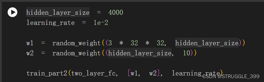
Train a Two-Layer Network
现在我们准备好运行训练循环了。 我们需要为全连接权重 w1 和 w2 显式分配张量。CIFAR 的每个小批量有 64 个示例,因此张量形状为 [64, 3, 32, 32]。展平后,x 形状应为 [64, 3 * 32 * 32]。 这将是 w1 第一个维度的大小。 w1 的第二个维度是隐藏层大小,这也是 w2 的第一个维度。最后,网络的输出是一个 10 维向量,表示 10 个类别的概率分布。您不需要调整任何超参数,但在训练一个 epoch 后,您应该会看到准确率高于 40%。
Iteration 0, loss = 3.4221
Checking accuracy on the val set
Got 126 / 1000 correct (12.60%)

Iteration 100, loss = 3.3836
Checking accuracy on the val set
Got 293 / 1000 correct (29.30%)

Iteration 200, loss = 2.4840
Checking accuracy on the val set
Got 350 / 1000 correct (35.00%)

Iteration 300, loss = 1.9273
Checking accuracy on the val set
Got 440 / 1000 correct (44.00%)

Iteration 400, loss = 2.0988
Checking accuracy on the val set
Got 391 / 1000 correct (39.10%)

Iteration 500, loss = 1.6173
Checking accuracy on the val set
Got 425 / 1000 correct (42.50%)

Iteration 600, loss = 1.7849
Checking accuracy on the val set
Got 452 / 1000 correct (45.20%)

Iteration 700, loss = 1.3852
Checking accuracy on the val set
Got 423 / 1000 correct (42.30%)
Training a ConvNet
在下面,您应该使用上面定义的函数在 CIFAR 上训练三层卷积网络。 该网络应具有以下架构:
- 具有 32 个 5x5 卷积核的卷积层(具有偏置),2 个零填充
- ReLU 非线性
- 具有 16 个 3x3 卷积核的卷积层(具有偏置),1 个零填充
- ReLU 非线性
- 全连接层(具有 bias)来计算 10 个类的得分
使用上面定义的 random_weight 函数初始化权重矩阵,并且应该使用上面的 zero_weight 函数初始化偏置向量。您不需要调整任何超参数,但如果一切正常,您应该在一个 epoch 后达到 42% 以上的准确率。
根据前面 three_layer_convnet 的推导,我们知道经过卷积层,其空间维度没有变化,变化的只是通道维度。
实现思路如下:
conv_w1参数的形状为:(32, 3, 5, 5),conv_b1的形状为:(32,)。conv_w2参数的形状为:(16, 32, 3, 3),conv_b2的形状为:(16,)。fc_w参数的形状为:(channel_2 * 32 * 32, 10),fc_b的形状为:(10,)。
learning_rate = 3e-3

channel_1 = 32
channel_2 = 16

conv_w1 = None
conv_b1 = None
conv_w2 = None
conv_b2 = None
fc_w = None
fc_b = None

################################################################################
# TODO: Initialize the parameters of a three-layer ConvNet.                    #
################################################################################
# *****START OF YOUR CODE (DO NOT DELETE/MODIFY THIS LINE)*****

conv_w1 = random_weight((channel_1, 3, 5, 5))
conv_w2 = random_weight((channel_2, channel_1, 3, 3))
conv_b1 = zero_weight((channel_1,))
conv_b2 = zero_weight((channel_2,))
fc_w = random_weight((channel_2 * 32 * 32, 10))
fc_b = zero_weight((10,))

# *****END OF YOUR CODE (DO NOT DELETE/MODIFY THIS LINE)*****
################################################################################
#                                 END OF YOUR CODE                             #
################################################################################

params = [conv_w1, conv_b1, conv_w2, conv_b2, fc_w, fc_b]
train_part2(three_layer_convnet, params, learning_rate)
测试结果如下:
Iteration 0, loss = 3.8523
Checking accuracy on the val set
Got 120 / 1000 correct (12.00%)

Iteration 100, loss = 1.8134
Checking accuracy on the val set
Got 343 / 1000 correct (34.30%)

Iteration 200, loss = 1.8792
Checking accuracy on the val set
Got 414 / 1000 correct (41.40%)

Iteration 300, loss = 1.7301
Checking accuracy on the val set
Got 426 / 1000 correct (42.60%)

Iteration 400, loss = 1.3870
Checking accuracy on the val set
Got 458 / 1000 correct (45.80%)

Iteration 500, loss = 1.5035
Checking accuracy on the val set
Got 475 / 1000 correct (47.50%)

Iteration 600, loss = 1.2601
Checking accuracy on the val set
Got 488 / 1000 correct (48.80%)

Iteration 700, loss = 1.5165
Checking accuracy on the val set
Got 484 / 1000 correct (48.40%)
PyTorch Module API
Barebone PyTorch 要求我们手动跟踪所有参数张量。这对于只有几个张量的小型网络来说没有问题,但如果要在大型网络中跟踪数十或数百个张量,就会非常不方便,而且容易出错。
PyTorch 提供的 nn.Module API 可以让你定义任意的网络架构,同时为你跟踪每一个可学习的参数。在第二部分,我们自己实现了 SGD。PyTorch 还提供了 torch.optim 包,它实现了所有常见的优化器,如 RMSProp、Adagrad 和 Adam。它甚至支持 L-BFGS 等近似二阶方法!关于每个优化器的具体规格,请参阅文档。
要使用 Module API,请按照以下步骤操作:
- 创建
nn.Module的子类。给网络类取一个直观的名字,如TwoLayerFC。 - 在构造函数
__init__()中,将所有需要的层定义为类属性。层对象(如nn.Linear和nn.Conv2d)本身就是nn.Module的子类,包含可学习的参数,因此你不必自己实例化原始张量,nn.Module会为你跟踪这些内部参数。请参阅文档,了解有关数十个内置层的更多信息。警告:别忘了先调用super().__init__()! - 在
forward()方法中,定义网络的连接性。应该使用__init__中定义的属性作为函数调用,将张量作为输入,并输出 "转换后 "的张量。不要在forward()中创建任何带有可学习参数的新层!所有这些参数都必须在__init__中预先声明。
下面是一个两层神经网络的例子:
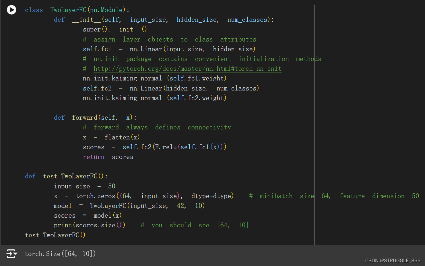
Three-Layer ConvNet
下面实现一个三层卷积神经网络,最后接上一个全连接层计算得分。网络的结构如下:
- Convolutional layer with
channel_15x5 filters with zero-padding of 2 - ReLU
- Convolutional layer with
channel_23x3 filters with zero-padding of 1 - ReLU
- Fully-connected layer to
num_classesclasses
使用 Kaiming 初始化方法初始化权重参数。提示:http://pytorch.org/docs/stable/nn.html#conv2d

实现思路为:
- 在
__init__()方法中实例化nn.Conv2d类创建卷积层,通过实例化nn.Linear类创建全连接层。 - 使用
nn.init.kaiming_normal_()方法初始化每一层的参数。 forward函数中定义网络的连接性。
class ThreeLayerConvNet(nn.Module):
    def __init__(self, in_channel, channel_1, channel_2, num_classes):
        super().__init__()
        ########################################################################
        # TODO: Set up the layers you need for a three-layer ConvNet with the  #
        # architecture defined above.                                          #
        ########################################################################
        # *****START OF YOUR CODE (DO NOT DELETE/MODIFY THIS LINE)*****

        self.conv1 = nn.Conv2d(in_channel, channel_1, 5, padding=2)
        nn.init.kaiming_normal_(self.conv1.weight)
        self.conv2 = nn.Conv2d(channel_1, channel_2, 3, padding=1)
        nn.init.kaiming_normal_(self.conv2.weight)
        self.fc3 = nn.Linear(channel_2 * 32 * 32, num_classes)
        nn.init.kaiming_normal_(self.fc3.weight)

        # *****END OF YOUR CODE (DO NOT DELETE/MODIFY THIS LINE)*****
        ########################################################################
        #                          END OF YOUR CODE                            #
        ########################################################################

    def forward(self, x):
        scores = None
        ########################################################################
        # TODO: Implement the forward function for a 3-layer ConvNet. you      #
        # should use the layers you defined in __init__ and specify the        #
        # connectivity of those layers in forward()                            #
        ########################################################################
        # *****START OF YOUR CODE (DO NOT DELETE/MODIFY THIS LINE)*****

        x = F.relu(self.conv1(x))
        x = F.relu(self.conv2(x))
        x = flatten(x)
        scores = self.fc3(x)

        # *****END OF YOUR CODE (DO NOT DELETE/MODIFY THIS LINE)*****
        ########################################################################
        #                             END OF YOUR CODE                         #
        ########################################################################
        return scores


def test_ThreeLayerConvNet():
    x = torch.zeros((64, 3, 32, 32), dtype=dtype)  # minibatch size 64, image size [3, 32, 32]
    model = ThreeLayerConvNet(in_channel=3, channel_1=12, channel_2=8, num_classes=10)
    scores = model(x)
    print(scores.size())  # you should see [64, 10]


test_ThreeLayerConvNet() # torch.Size([64, 10])
Check Accuracy
有了验证集或测试集,我们就可以检查神经网络的分类准确性。这个版本与 check_accuracy_part2 略有不同。不再需要手动输入参数。
Training Loop
Train a Two-Layer Network
现在我们可以运行训练循环了。与 Barebone Pytorch 部分相比,我们不再明确分配参数张量。只需将输入大小、隐藏层大小和类的数量(即输出大小)传递给 TwoLayerFC 的构造函数即可。还需要定义一个优化器,用于跟踪 TwoLayerFC 中的所有可学习参数。不需要调整任何超参数,但在训练一个 epoch 后,你应该能看到模型准确率超过 40%。

测试结果如下:
Iteration 0, loss = 3.3450
Checking accuracy on validation set
Got 144 / 1000 correct (14.40)

Iteration 100, loss = 2.7940
Checking accuracy on validation set
Got 316 / 1000 correct (31.60)

Iteration 200, loss = 2.2455
Checking accuracy on validation set
Got 374 / 1000 correct (37.40)

Iteration 300, loss = 1.8478
Checking accuracy on validation set
Got 379 / 1000 correct (37.90)

Iteration 400, loss = 1.6748
Checking accuracy on validation set
Got 406 / 1000 correct (40.60)

Iteration 500, loss = 1.9785
Checking accuracy on validation set
Got 407 / 1000 correct (40.70)

Iteration 600, loss = 1.9285
Checking accuracy on validation set
Got 431 / 1000 correct (43.10)

Iteration 700, loss = 1.8859
Checking accuracy on validation set
Got 435 / 1000 correct (43.50)
Train a Three-Layer ConvNet
learning_rate = 3e-3
channel_1 = 32
channel_2 = 16

model = None
optimizer = None
################################################################################
# TODO: Instantiate your ThreeLayerConvNet model and a corresponding optimizer #
################################################################################
# *****START OF YOUR CODE (DO NOT DELETE/MODIFY THIS LINE)*****

model = ThreeLayerConvNet(3, channel_1, channel_2, 10)
optimizer = optim.SGD(model.parameters(), lr=learning_rate)

# *****END OF YOUR CODE (DO NOT DELETE/MODIFY THIS LINE)*****
################################################################################
#                                 END OF YOUR CODE                             #
################################################################################

train_part34(model, optimizer)
测试结果如下:
Iteration 0, loss = 3.0369
Checking accuracy on validation set
Got 92 / 1000 correct (9.20)

Iteration 100, loss = 1.8400
Checking accuracy on validation set
Got 317 / 1000 correct (31.70)

Iteration 200, loss = 1.6443
Checking accuracy on validation set
Got 399 / 1000 correct (39.90)

Iteration 300, loss = 1.6305
Checking accuracy on validation set
Got 424 / 1000 correct (42.40)

Iteration 400, loss = 1.6039
Checking accuracy on validation set
Got 426 / 1000 correct (42.60)

Iteration 500, loss = 1.8652
Checking accuracy on validation set
Got 458 / 1000 correct (45.80)

Iteration 600, loss = 1.5585
Checking accuracy on validation set
Got 467 / 1000 correct (46.70)

Iteration 700, loss = 1.4178
Checking accuracy on validation set
Got 469 / 1000 correct (46.90)
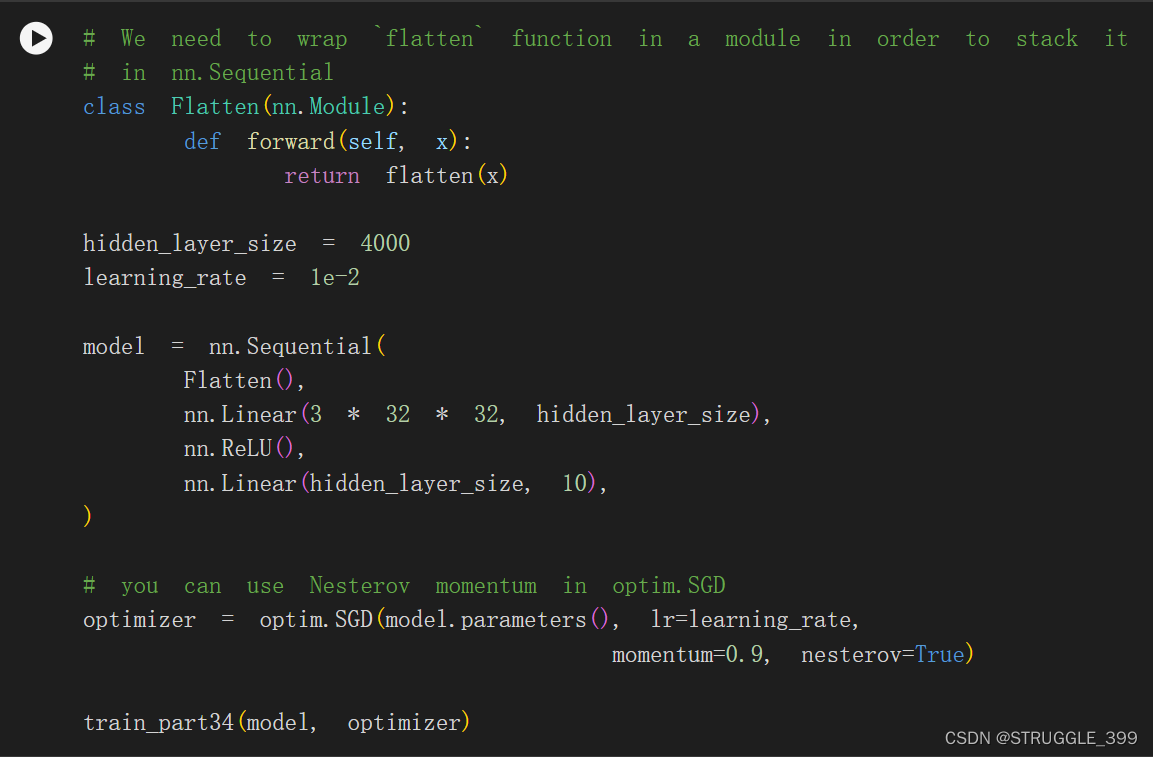
PyTorch Sequential API
对于像堆叠前馈层这样的简单模型,你仍然需要经过 3 个步骤:子类 nn.Module、在 __init__ 中将层分配给类属性、在 forward() 中逐个调用每个层。有没有更方便的方法?
幸运的是,PyTorch 提供了一个名为 nn.Sequential 的容器模块,它将上述步骤合二为一。它没有 nn.Module 那么灵活,因为你不能指定比堆叠前馈层更复杂的拓扑结构,但对于许多用例来说,它已经足够好了。
Two-Layer Network
让我们看看如何使用 nn.Sequential 重写我们的双层全连接网络示例,并使用上面定义的训练循环对其进行训练。同样,在这里不需要调整任何超参数,但在训练一个 epoch 后,准确率应达到 40% 以上。
测试结果如下:
Iteration 0, loss = 2.3934
Checking accuracy on validation set
Got 150 / 1000 correct (15.00)

Iteration 100, loss = 1.9008
Checking accuracy on validation set
Got 384 / 1000 correct (38.40)

Iteration 200, loss = 1.7565
Checking accuracy on validation set
Got 389 / 1000 correct (38.90)

Iteration 300, loss = 2.0154
Checking accuracy on validation set
Got 413 / 1000 correct (41.30)

Iteration 400, loss = 1.5038
Checking accuracy on validation set
Got 430 / 1000 correct (43.00)

Iteration 500, loss = 1.8432
Checking accuracy on validation set
Got 425 / 1000 correct (42.50)

Iteration 600, loss = 1.6545
Checking accuracy on validation set
Got 438 / 1000 correct (43.80)

Iteration 700, loss = 1.7530
Checking accuracy on validation set
Got 430 / 1000 correct (43.00)
Three-Layer ConvNet
在这里,您应该使用 nn.Sequential 来定义和训练一个三层 ConvNet,其架构与我们在 PyTorch Module API 部分中使用的相同:
- Convolutional layer (with bias) with 32 5x5 filters, with zero-padding of 2
- ReLU
- Convolutional layer (with bias) with 16 3x3 filters, with zero-padding of 1
- ReLU
- Fully-connected layer (with bias) to compute scores for 10 classes
您可以使用默认的 PyTorch 权重初始化。你应该使用随机梯度下降法优化你的模型,Nesterov 动量为 0.9。同样,你不需要调整任何超参数,但在训练一个 epoch 后,你应该能看到高于 55% 的准确率。
channel_1 = 32
channel_2 = 16
learning_rate = 1e-2

model = None
optimizer = None

################################################################################
# TODO: Rewrite the 3-layer ConvNet with bias from Part III with the           #
# Sequential API.                                                              #
################################################################################
# *****START OF YOUR CODE (DO NOT DELETE/MODIFY THIS LINE)*****

model = nn.Sequential(
    nn.Conv2d(3, channel_1, 5, padding=2),
    nn.ReLU(),
    nn.Conv2d(channel_1, channel_2, 3, padding=1),
    nn.ReLU(),
    Flatten(),
    nn.Linear(channel_2 * 32 * 32, 10)
)

optimizer = optim.SGD(model.parameters(), lr=learning_rate, momentum=0.9, nesterov=True)

# *****END OF YOUR CODE (DO NOT DELETE/MODIFY THIS LINE)*****
################################################################################
#                                 END OF YOUR CODE                             #
################################################################################

train_part34(model, optimizer)
测试结果如下:
Iteration 0, loss = 2.3133
Checking accuracy on validation set
Got 119 / 1000 correct (11.90)

Iteration 100, loss = 1.4949
Checking accuracy on validation set
Got 459 / 1000 correct (45.90)

Iteration 200, loss = 1.5431
Checking accuracy on validation set
Got 469 / 1000 correct (46.90)

Iteration 300, loss = 1.2729
Checking accuracy on validation set
Got 497 / 1000 correct (49.70)

Iteration 400, loss = 1.3262
Checking accuracy on validation set
Got 539 / 1000 correct (53.90)

Iteration 500, loss = 1.2056
Checking accuracy on validation set
Got 565 / 1000 correct (56.50)

Iteration 600, loss = 1.2764
Checking accuracy on validation set
Got 562 / 1000 correct (56.20)

Iteration 700, loss = 1.3684
Checking accuracy on validation set
Got 583 / 1000 correct (58.30)
CIFAR-10 open-ended challenge
这一部分应该算是 Q5 最有趣的一个部分,前面简要地向我们介绍了 Tensor、Barebone PyTorch、Module API、Sequential API。我们在这里可以尝试各种各样的网络结构。
现在,我们的任务是试验各种架构、超参数、损失函数和优化器,训练出一个模型,在 10 个历元内,在 CIFAR-10 验证集上达到至少 70% 的准确率。您可以使用上面的 check_accuracy 和 train 函数。您可以使用 nn.Module 或 nn.Sequential API。
以下是每个组件的官方 API 文档。需要注意的是:我们在 "Spatial batch norm "类中使用的名称在 PyTorch 中叫做 “BatchNorm2D”。
torch.nn中的层:http://pytorch.org/docs/stable/nn.html- 激活函数:http://pytorch.org/docs/stable/nn.html#non-linear-activations
- 损失函数:http://pytorch.org/docs/stable/nn.html#loss-functions
- 优化器:http://pytorch.org/docs/stable/optim.html
我们应该尝试的:
- filter size:上面我们使用的是 5x5;更小的过滤器会更有效吗?
- Number of filters:以上我们使用了 32 个过滤器。使用更多或更少的滤波器效果更好吗?
- Pooling vs Strided Convolution:是使用最大池化还是仅使用跨距卷积?
- Batch Normalization:尝试在卷积层后添加 Spatial Batch Normalization,在仿射层后添加 Batch Normalization。你的网络是否训练得更快?
- Network architecture:上述网络有两层可训练参数。你能用深度网络做得更好吗?可以尝试的架构包括:
- [conv-relu-pool]xN -> [affine]xM -> [softmax 或 SVM]
- [conv-relu-conv-relu-pool]xN -> [affine]xM -> [softmax 或 SVM]
- [batchnorm-relu-conv]xN -> [affine]xM -> [softmax 或 SVM]
- Global Average Pooling:与其先进行扁平化处理,然后建立多个仿射层,不如先进行卷积,直到图像变小(7x7 左右),然后执行平均池化操作,得到 1x1 的图像图片(1, 1 , Filter#),再将其重塑为 (Filter#) 向量。谷歌的 Inception 网络就采用了这种方法(其架构见表 1)
- Regularization:添加 L2 权重正则化,或者使用 Dropout。
Model 1
第一个模型的结构如下:
[conv-relu-pool]x4->[affine-dropout]x2->affine->Softmax
代码如下:
################################################################################
# TODO:                                                                        #
# Experiment with any architectures, optimizers, and hyperparameters.          #
# Achieve AT LEAST 70% accuracy on the *validation set* within 10 epochs.      #
#                                                                              #
# Note that you can use the check_accuracy function to evaluate on either      #
# the test set or the validation set, by passing either loader_test or         #
# loader_val as the second argument to check_accuracy. You should not touch    #
# the test set until you have finished your architecture and  hyperparameter   #
# tuning, and only run the test set once at the end to report a final value.   #
################################################################################
model = None
optimizer = None

# *****START OF YOUR CODE (DO NOT DELETE/MODIFY THIS LINE)*****
model = nn.Sequential(
    nn.Conv2d(3, 16, kernel_size=3, padding=1),
    nn.ReLU(),
    nn.MaxPool2d(kernel_size=2, stride=2),
    nn.Conv2d(16, 32, kernel_size=3, padding=1),
    nn.ReLU(),
    nn.MaxPool2d(kernel_size=2, stride=2),
    nn.Conv2d(32, 64, kernel_size=3, padding=1),
    nn.ReLU(),
    nn.MaxPool2d(kernel_size=2, stride=2),
    nn.Conv2d(64, 128, kernel_size=3, padding=1),
    nn.ReLU(),
    nn.MaxPool2d(kernel_size=2, stride=2),
    Flatten(),
    nn.Linear(512, 4096),
    nn.Dropout(),
    nn.Linear(4096, 4096),
    nn.Dropout(),
    nn.Linear(4096, 10)
)

optimizer = optim.SGD(model.parameters(), lr=1e-3, momentum=0.9, nesterov=True)

# *****END OF YOUR CODE (DO NOT DELETE/MODIFY THIS LINE)*****
################################################################################
#                                 END OF YOUR CODE                             #
################################################################################

# You should get at least 70% accuracy.
# You may modify the number of epochs to any number below 15.
train_part34(model, optimizer, epochs=10)
测试结果如下:
Model 2
第二个网络的结构如下:
[conv-batchnorm-relu-conv-batchnorm-relu-pool]x3->[affine-dropout]x2->affine->Softmax
核心代码如下:
model = nn.Sequential(
    nn.Conv2d(3, 64, kernel_size=3, padding=1),
    nn.BatchNorm2d(64),
    nn.ReLU(),
    nn.Conv2d(64, 64, kernel_size=3, padding=1),
    nn.BatchNorm2d(64),
    nn.ReLU(),
    nn.MaxPool2d(kernel_size=2, stride=2),
    nn.Conv2d(64, 128, kernel_size=3, padding=1),
    nn.BatchNorm2d(128),
    nn.ReLU(),
    nn.Conv2d(128, 128, kernel_size=3, padding=1),
    nn.BatchNorm2d(128),
    nn.ReLU(),
    nn.MaxPool2d(kernel_size=2, stride=2),
    nn.Conv2d(128, 256, kernel_size=3, padding=1),
    nn.BatchNorm2d(256),
    nn.ReLU(),
    nn.Conv2d(256, 256, kernel_size=3, padding=1),
    nn.BatchNorm2d(256),
    nn.ReLU(),
    nn.MaxPool2d(kernel_size=2, stride=2),
    Flatten(),
    nn.Linear(4096, 4096),
    nn.Dropout(),
    nn.Linear(4096, 4096),
    nn.Dropout(),
    nn.Linear(4096, 10)
)

optimizer = optim.SGD(model.parameters(), lr=3e-3, momentum=0.9, nesterov=True)
测试结果如下:

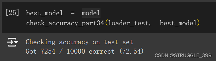
此外,还可以尝试更多的优化器,例如:AdaGrad、RMSProp、Adam。尝试更多的激活函数,例如:Leaky ReLU、PReLU、ELU等等。还可以尝试新的网络结构,例如 ResNet、DenseNet。


 1313
1313


 被折叠的 条评论
为什么被折叠?
被折叠的 条评论
为什么被折叠?
 到【灌水乐园】发言


