SVM向量机及人脸特征提取

最新推荐文章于 2022-01-16 18:48:34 发布

@川川而山

最新推荐文章于 2022-01-16 18:48:34 发布

阅读量1.4k

点赞数 4

文章标签：支持向量机机器学习人工智能

本文链接：https://blog.csdn.net/weixin_47306453/article/details/121278461

版权

文章目录

一、SVM向量机
二、人脸特征提取
- 1.win10安装opencv和dlib
- 2.打开摄像头，实时采集人脸并保存、绘制68个特征点
三、参考链接

一、SVM向量机

1.向量机简述

（1）简介： 支持向量机(support vector machine, SVM)：是监督学习中最有影响力的方法之一。类似于逻辑回归，这个模型也是基于线性函数wTx+b的。不同于逻辑回归的是，支持向量机不输出概率，只输出类别。当wTx+b为正时，支持向量机预测属于正类。类似地，当wTx+b为负时，支持向量机预测属于负类。

（2）工作原理：将数据映射到高维特征空间，这样即使数据不是线性可分，也可以对该数据点进行分类。

作用：进行线性分类之外，SVM还可以使用所谓的核技巧有效地进行非线性分类，将其输入隐式映射到高维特征空间中。

SVM对偶形式的求解公式为

在这里插入图片描述

2.核函数简述

核函数原理：将原始非线性的样本通过非线性映射映射至高维特征空间，使得在新的空间里样本线性可分，进而可用线性样本的分类理论解决此类问题。

核函数：包括齐次多项式、非齐次多项式、双曲正切、高斯核(Gaussiankernel)、线性核、径向基函数(radialbasis function, RBF)核和、Sigmoid核。

优点 ：

1）核函数的引入避免了“维数灾难”,大大减小了计算量。而输入空间的维数n对核函数矩阵无影响，因此，核函数方法可以有效处理高维输入。
2）无需知道非线性变换函数Φ的形式和参数.
3）核函数的形式和参数的变化会隐式地改变从输入空间到特征空间的映射，进而对
特征空间的性质产生影响，最终改变各种核函数方法的性能。
4）核函数方法可以和不同的算法相结合，形成多种不同的基于核函数技术的方法，
且这两部分的设计可以单独进行，并可以为不同的应用选择不同的核函数和算法。

3.鸢尾花数据集

（1）数据基础处理
导入相关包

import numpy as np
from sklearn import datasets   #导入数据集
import matplotlib.pyplot as plt  
from sklearn.preprocessing import StandardScaler
from matplotlib.colors import ListedColormap

绘制边界函数

import numpy as np
from sklearn import datasets   #导入数据集
import matplotlib.pyplot as plt  
from sklearn.preprocessing import StandardScaler
from matplotlib.colors import ListedColormap

导入测试数据并进行预处理

def plot_decision_boundary(model,axis):
    x0,x1=np.meshgrid(
        np.linspace(axis[0],axis[1],int((axis[1]-axis[0])*100)).reshape(-1,1),
        np.linspace(axis[2],axis[3],int((axis[3]-axis[2])*100)).reshape(-1,1))
    # meshgrid函数是从坐标向量中返回坐标矩阵
    x_new=np.c_[x0.ravel(),x1.ravel()]
    y_predict=model.predict(x_new)#获取预测值
    zz=y_predict.reshape(x0.shape)
    custom_cmap=ListedColormap(['#EF9A9A','#FFF59D'])
    plt.contourf(x0,x1,zz,cmap=custom_cmap)
iris = datasets.load_iris()
data_x = iris.data[:, :2] 
data_y = iris.target
scaler=StandardScaler()# 标准化
data_x = scaler.fit_transform(data_x)#计算训练数据的均值和方差

绘制基本鸢尾花数据集

  plt.rcParams["font.sans-serif"] = ['SimHei']    # 用来正常显示中文标签，SimHei是字体名称，字体必须在系统中存在，字体的查看方式和安装第三部分
plt.rcParams['axes.unicode_minus'] = False     # 用来正常显示负号
plt.scatter(data_x[data_y==0, 0],data_x[data_y==0, 1])    # 选取y所有为0的+X的第一列
plt.scatter(data_x[data_y==1, 0],data_x[data_y==1, 1])    # 选取y所有为1的+X的第一列

plt.xlabel('sepal length')    # 设置横坐标标注xlabel为sepal width
plt.ylabel('sepal width')    # 设置纵坐标标注ylabel为sepal length
plt.title('sepal散点图')    # 设置散点图的标题为sepal散点图
plt.show()

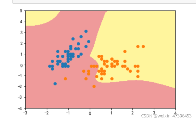
3.多项式分类函数

多项式核进行处理

from sklearn.preprocessing import PolynomialFeatures #导入多项式回归
from sklearn.pipeline import Pipeline #导入python里的管道
from sklearn.svm import LinearSVC
def PolynomialSVC(degree,c=5):#多项式svm
    """
    :param d:阶数
    :param C:正则化常数
    :return:一个Pipeline实例
    """
    return Pipeline([
            # 将源数据 映射到 3阶多项式
            ("poly_features", PolynomialFeatures(degree=degree)),
            # 标准化
            ("scaler", StandardScaler()),
            # SVC线性分类器
            ("svm_clf", LinearSVC(C=c, loss="hinge", random_state=10,max_iter=100000))
        ])

poly_svc=PolynomialSVC(degree=5)
poly_svc.fit(data_x,data_y)
plot_decision_boundary(poly_svc,axis=[-3,4,-4,5])
plt.scatter(data_x[data_y==0,0],data_x[data_y==0,1])
plt.scatter(data_x[data_y==2,0],data_x[data_y==2,1])
plt.show()

在这里插入图片描述

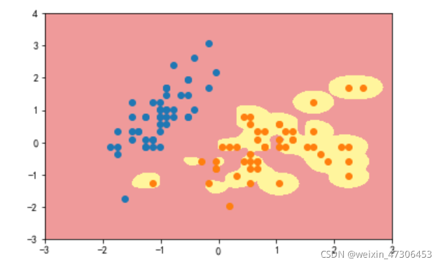
4.高斯核方式

定义RBF核的SVM函数
y=1（只需要修改gamma的值即可）

from sklearn.svm import SVC #导入svm
def RBFKernelSVC(gamma=1.0):
    return Pipeline([
        ('std_scaler',StandardScaler()),
        ('svc',SVC(kernel='rbf',gamma=gamma))
    ])
svc=RBFKernelSVC(gamma=42)#gamma参数很重要，gamma参数越大，支持向量越小
svc.fit(data_x,data_y)
plot_decision_boundary(svc,axis=[-3,3,-3,4])
plt.scatter(data_x[data_y==0,0],data_x[data_y==0,1])
plt.scatter(data_x[data_y==2,0],data_x[data_y==2,1])
plt.show()

在这里插入图片描述
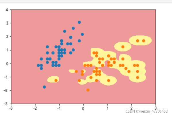
gamma=10

gamma=100

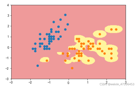
可以看到，γ 取值越大，就是高斯分布的钟形图越窄，这里相当于每个样本点都形成了钟形图。很明显这样是过拟合的

5.月亮数据集

多项式分类函数
导入需要的包和月亮数据集并进行处理可视化

import numpy as np
import matplotlib.pyplot as plt
from sklearn import datasets
from sklearn.preprocessing import PolynomialFeatures,StandardScaler
from sklearn.svm import LinearSVC
from sklearn.pipeline import Pipeline
from sklearn.svm import SVC
X, y = datasets.make_moons() #使用生成的数据
#print(X.shape) # (100,2)
#print(y.shape) # (100,)
plt.scatter(X[y==0,0],X[y==0,1]) 
plt.scatter(X[y==1,0],X[y==1,1])
plt.show()

在这里插入图片描述
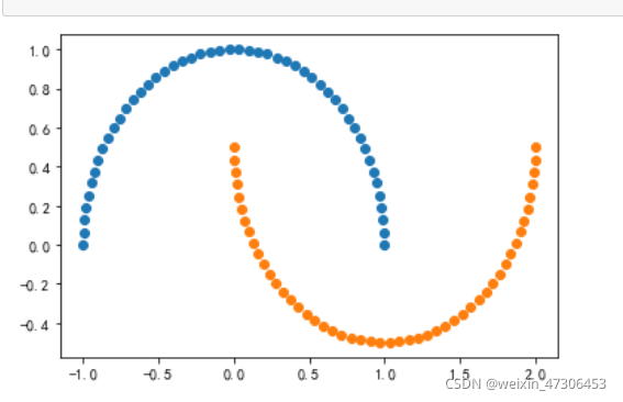
生成噪声点（数据集中的干扰数据（对场景描述不准确的数据），即测量变量中的随机误差或方差）并实现可视化。

X, y = datasets.make_moons(noise=0.15,random_state=777) #随机生成噪声点，random_state是随机种子，noise是方差
plt.scatter(X[y==0,0],X[y==0,1]) 
plt.scatter(X[y==1,0],X[y==1,1])
plt.show()

在这里插入图片描述
定义非线性SVM函数

def PolynomialSVC(degree,C=1.0):
    return Pipeline([
        ("poly",PolynomialFeatures(degree=degree)),#生成多项式
        ("std_scaler",StandardScaler()),#标准化
        ("linearSVC",LinearSVC(C=C))#最后生成svm
    ])

调用PolynomialSVC函数进行分类可视化
调用非线性SVM分类，实例化SVC

# 边界绘制函数
def plot_decision_boundary(model,axis):
    x0,x1=np.meshgrid(
        np.linspace(axis[0],axis[1],int((axis[1]-axis[0])*100)).reshape(-1,1),
        np.linspace(axis[2],axis[3],int((axis[3]-axis[2])*100)).reshape(-1,1))
    # meshgrid函数是从坐标向量中返回坐标矩阵
    x_new=np.c_[x0.ravel(),x1.ravel()]
    y_predict=model.predict(x_new)#获取预测值
    zz=y_predict.reshape(x0.shape)
    custom_cmap=ListedColormap(['#EF9A9A','#FFF59D','#90CAF9'])
    plt.contourf(x0,x1,zz,cmap=custom_cmap)
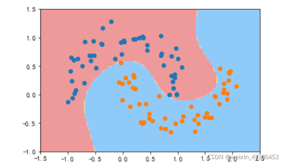
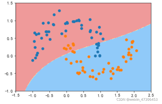
poly_svc = PolynomialSVC(degree=5)
poly_svc.fit(X,y)
plot_decision_boundary(poly_svc,axis=[-1.5,2.5,-1.0,1.5])
plt.scatter(X[y==0,0],X[y==0,1]) 
plt.scatter(X[y==1,0],X[y==1,1])
plt.show()

在这里插入图片描述
进行核处理

def PolynomialKernelSVC(degree,C=1.0):
    return Pipeline([
        ("std_scaler",StandardScaler()),
        ("kernelSVC",SVC(kernel="poly")) # poly代表多项式特征
    ])
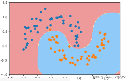
poly_kernel_svc = PolynomialKernelSVC(degree=5)
poly_kernel_svc.fit(X,y)
plot_decision_boundary(poly_kernel_svc,axis=[-1.5,2.5,-1.0,1.5])
plt.scatter(X[y==0,0],X[y==0,1]) 
plt.scatter(X[y==1,0],X[y==1,1])
plt.show()

在这里插入图片描述
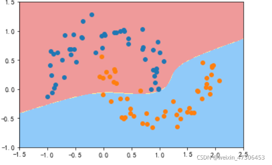
可以看到已经非常接近线性了

6.高斯核方式

导入需要的包和月亮数据集并输出

import numpy as np
import matplotlib.pyplot as plt
from sklearn import datasets
from sklearn.preprocessing import StandardScaler
from sklearn.svm import SVC
from sklearn.pipeline import Pipeline
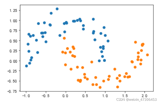
X,y = datasets.make_moons(noise=0.15,random_state=777)
plt.scatter(X[y==0,0],X[y==0,1])
plt.scatter(X[y==1,0],X[y==1,1])
plt.show()

在这里插入图片描述
定义RBF核的SVM函数
并且实例化向γ传递参
y=0.1：

from sklearn.preprocessing import StandardScaler
from sklearn.svm import SVC
from sklearn.pipeline import Pipeline
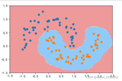
def RBFKernelSVC(gamma=0.1):
    return Pipeline([ ('std_scaler',StandardScaler()), ('svc',SVC(kernel='rbf',gamma=gamma)) ])
svc = RBFKernelSVC()
svc.fit(X,y)
plot_decision_boundary(svc,axis=[-1.5,2.5,-1.0,1.5])
plt.scatter(X[y==0,0],X[y==0,1])
plt.scatter(X[y==1,0],X[y==1,1])
plt.show()

在这里插入图片描述
gamma=1

gamma=10

gamma=100

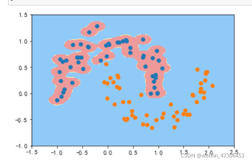
可以看到，γ 取值越大，就是高斯分布的钟形图越窄，这里相当于每个样本点都形成了钟形图。很明显这样是过拟合的

二、人脸特征提取

1.win10安装opencv和dlib

（1）anaconda下载

https://blog.csdn.net/ITLearnHall/article/details/81708148
配置anaconda环境变量

（2）使用python命令查看当前版本
.搜索对应版本的dlib文件下载好后用命令在适合的位置进行安装
python3.8的链接：
https://pan.baidu.com/s/1kLn0uEqO5xinuTMZzk3fFA
提取码：kh99
输入命令下载dlib

pip install +下载的dilb路径
dilb只能放在其中一个磁盘的当前目录下，如D\

（3）使用命令安装opencv

 pip3 install opencv_python

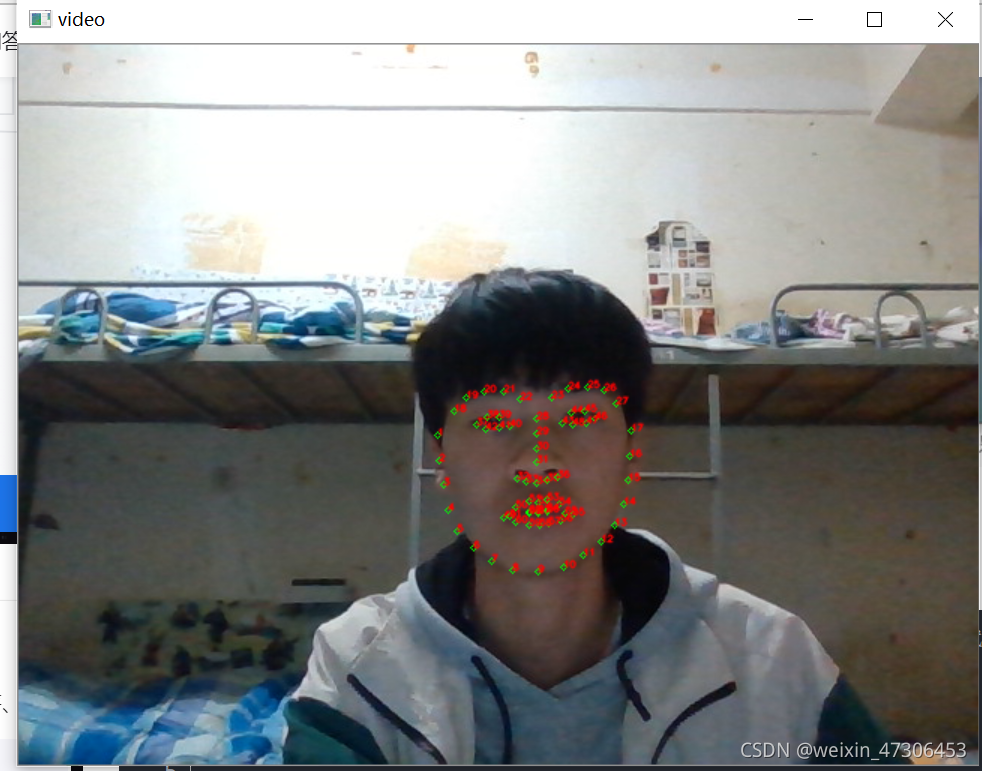
2.打开摄像头，实时采集人脸并保存、绘制68个特征点

# -*- coding: utf-8 -*-
"""
Created on Wed Oct 27 03:15:10 2021

@author: GT72VR
"""
import numpy as np
import cv2
import dlib
import os
import sys
import random
# 存储位置
output_dir = 'C:/Users/86199/tvcamera'
size = 64
 
if not os.path.exists(output_dir):
    os.makedirs(output_dir)
# 改变图片的亮度与对比度
 
def relight(img, light=1, bias=0):
    w = img.shape[1]
    h = img.shape[0]
    #image = []
    for i in range(0,w):
        for j in range(0,h):
            for c in range(3):
                tmp = int(img[j,i,c]*light + bias)
                if tmp > 255:
                    tmp = 255
                elif tmp < 0:
                    tmp = 0
                img[j,i,c] = tmp
    return img
 
#使用dlib自带的frontal_face_detector作为我们的特征提取器
detector = dlib.get_frontal_face_detector()
# 打开摄像头 参数为输入流，可以为摄像头或视频文件
camera = cv2.VideoCapture(0)
#camera = cv2.VideoCapture('C:/Users/CUNGU/Videos/Captures/wang.mp4')
ok = True

detector = dlib.get_frontal_face_detector()
predictor = dlib.shape_predictor('shape_predictor_68_face_landmarks.dat')


while ok:
    # 读取摄像头中的图像，ok为是否读取成功的判断参数
    ok, img = camera.read()
    
    # 转换成灰度图像
    img_gray = cv2.cvtColor(img, cv2.COLOR_BGR2GRAY)

    rects = detector(img_gray, 0)
    
    for i in range(len(rects)):
        landmarks = np.matrix([[p.x, p.y] for p in predictor(img,rects[i]).parts()])
        for idx, point in enumerate(landmarks):
            # 68点的坐标
            pos = (point[0, 0], point[0, 1])
            print(idx,pos)
    
            # 利用cv2.circle给每个特征点画一个圈，共68个
            cv2.circle(img, pos, 2, color=(0, 255, 0))
            # 利用cv2.putText输出1-68
            font = cv2.FONT_HERSHEY_SIMPLEX
            cv2.putText(img, str(idx+1), pos, font, 0.2, (0, 0, 255), 1,cv2.LINE_AA)
    cv2.imshow('video', img)
    k = cv2.waitKey(1)
    if k == 27:    # press 'ESC' to quit
        break
    
camera.release()
cv2.destroyAllWindows()

在这里插入图片描述

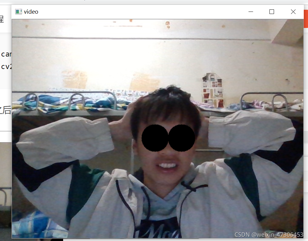
人脸虚拟P上一付墨镜
首先导入代码需要用到的包

# 导入包
import numpy as np
import cv2
import dlib
import os
import sys
import random

添加函数，获得默认的人脸检测器和训练好的68特征点检测器

def get_detector_and_predicyor():
    #使用dlib自带的frontal_face_detector作为我们的特征提取器
    detector = dlib.get_frontal_face_detector()
    """
    功能：人脸检测画框
    参数：PythonFunction和in Classes
    in classes表示采样次数，次数越多获取的人脸的次数越多，但更容易框错
    返回值是矩形的坐标，每个矩形为一个人脸（默认的人脸检测器）
    """
    #返回训练好的人脸68特征点检测器
    predictor = dlib.shape_predictor('shape_predictor_68_face_landmarks.dat')
    return detector,predictor
#获取检测器
detector,predictor=get_detector_and_predicyor()

添加给眼睛画圆的函数，这个就是找到眼睛周围的特征点，然后确认中心点，后面用cirecle函数画出来就行了

def painting_sunglasses(img,detector,predictor):   
    #给人脸带上墨镜
    rects = detector(img_gray, 0)  
    for i in range(len(rects)):
        landmarks = np.matrix([[p.x, p.y] for p in predictor(img,rects[i]).parts()])
        right_eye_x=0
        right_eye_y=0
        left_eye_x=0
        left_eye_y=0
        for i in range(36,42):#右眼范围
            #将坐标相加
            right_eye_x+=landmarks[i][0,0]
            right_eye_y+=landmarks[i][0,1]
        #取眼睛的中点坐标
        pos_right=(int(right_eye_x/6),int(right_eye_y/6))
        """
        利用circle函数画圆
        函数原型      
        cv2.circle(img, center, radius, color[, thickness[, lineType[, shift]]])
        img：输入的图片data
        center：圆心位置
        radius：圆的半径
        color：圆的颜色
        thickness：圆形轮廓的粗细（如果为正）。负厚度表示要绘制实心圆。
        lineType： 圆边界的类型。
        shift：中心坐标和半径值中的小数位数。
        """
        cv2.circle(img=img, center=pos_right, radius=30, color=(0,0,0),thickness=-1)
        for i in range(42,48):#左眼范围
           #将坐标相加
            left_eye_x+=landmarks[i][0,0]
            left_eye_y+=landmarks[i][0,1]
        #取眼睛的中点坐标
        pos_left=(int(left_eye_x/6),int(left_eye_y/6))
        cv2.circle(img=img, center=pos_left, radius=30, color=(0,0,0),thickness=-1)

最后调用画圆的函数

camera = cv2.VideoCapture(0)#打开摄像头
ok=True
# 打开摄像头 参数为输入流，可以为摄像头或视频文件
while ok:
    ok,img = camera.read()
     # 转换成灰度图像
    img_gray = cv2.cvtColor(img,cv2.COLOR_BGR2GRAY)
    #display_feature_point(img,detector,predictor)
    painting_sunglasses(img,detector,predictor)#调用画墨镜函数
    cv2.imshow('video', img)
    k = cv2.waitKey(1)
    if k == 27:    # press 'ESC' to quit
        break
camera.release()
cv2.destroyAllWindows()

在这里插入图片描述

三、参考链接

https://blog.csdn.net/fengbingchun/article/details/78326704

https://blog.csdn.net/weixin_47554309/article/details/121120120

https://blog.csdn.net/qq_46689721/article/details/121254232?spm=1001.2014.3001.5501

https://blog.csdn.net/qq_46689721/article/details/121273562?spm=1001.2014.3001.5501

@川川而山

关注

4
点赞
踩
7

收藏

觉得还不错? 一键收藏
0
评论
SVM向量机及人脸特征提取

文章目录一、SVM向量机1.向量机简述2.核函数简述3.鸢尾花数据集3.多项式分类函数4.高斯核方式5.月亮数据集6.高斯核方式二、人脸特征提取1.win10安装opencv和dlib2.打开摄像头，实时采集人脸并保存、绘制68个特征点三、参考链接一、SVM向量机1.向量机简述（1）简介：支持向量机(support vector machine, SVM)：是监督学习中最有影响力的方法之一。类似于逻辑回归，这个模型也是基于线性函数wTx+b的。不同于逻辑回归的是，支持向量机不输出概率，只输出类别。当
复制链接

扫一扫