手写数字识别，吴恩达机器学习

吴恩达机器学习之手写数字识别——logistic回归

本部分主要是通过logistic回归解决多分类问题，对每一个维度建立对应的logistic回归方程，对每一个结果值进行预测，最大的概率值即为可能的结果。

数据集介绍

数据集下载地址，在下面的博客链接可以下载：
https://blog.csdn.net/weixin_47598128/article/details/139394307?spm=1001.2014.3001.5501

数据集为0-9的手写数字，下面进行数据加载并进行具体介绍：

import numpy as np
import matplotlib.pyplot as plt
import pandas as pd
from scipy.io import loadmat
import scipy.optimize as opt

# 加载数据
path = "ex3data1.mat"
data = loadmat(path)  # 返回一个字典
# print(data.keys())
x = data['X']
y = np.array(data['y'])
print(x.shape, y.shape)
print(np.unique(y))

# output
# (5000, 400) (5000, 1)
# [ 1  2  3  4  5  6  7  8  9 10]

数据类型为mat，这是MATLAB的一种输出数据类型，其中存放的数据按照索引名称，可以理解为存放的为数组。

X：代表5000个手写数字图像，一个图像为一个1400的矩阵，为一个2020矩阵扁平化的结果。
Y：对手写数字图像的预测值，其中1-9的预测值为对应的数组，而0的预测值被映射为10，或许和我们的思维方式有些不同，但是这对模型训练和结果预测并没有影响。

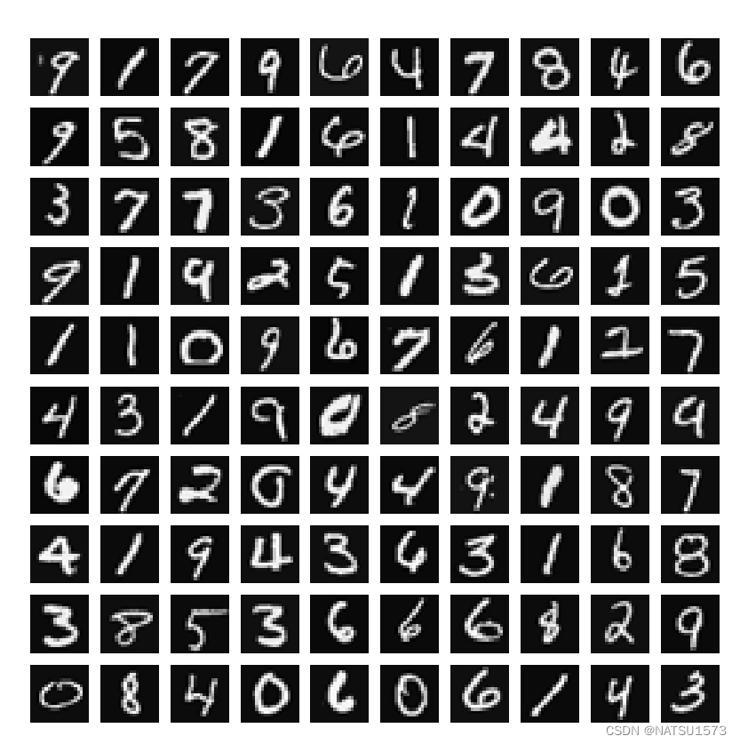
输入数据转化成图像，展示其中的一百个如下：

# 显示部分数据
sample_idx = np.random.choice(np.arange(x.shape[0]), 100, replace=False)
sample_images = x[sample_idx, :]
print(sample_images.shape)
pic_sample(sample_images)

def pic_sample(x):
    fig, axs = plt.subplots(10, 10, figsize=(10, 10))
    for i,ax in enumerate(axs.flat):
        ax.imshow(x[i, :].reshape(20, 20).T, cmap='gray')
        ax.axis('off')
    plt.show()
    input()

模型训练

在了解了输入数据之后，下面需要进行模型创建。

相较于传统的二分类问题，手写数字识别为一个“十分类”问题，也就是类别是10个，我们无法像二分类问题一样，建立一个logistic方程来实现分类；而需要创建10个logistic方程。

损失函数

损失函数的定义和二分类问题一样：
$cost=\frac{1}{m}{\sum }_{i=1}^m(-y\lg h_{\theta }(x^i)-(1-y)\lg 1-h_{\theta }(x))+lr\ast \frac{1}{2m}{\sum }_{j=1}^n{\theta }_j^2$

在程序实现中，需要重点考虑输入，输出的维度关系：

def sigmoid(z):
    return 1 / (1 + np.exp(-z))

def cost_function(theta, X, y,lr):
    hx = sigmoid(np.dot(X,theta))# (n,)
    left = -np.dot(y.T, np.log(hx))
    right = -np.dot((1-y).T, np.log(1-hx))
    reg = lr*np.sum(theta[1:]*theta[1:])
    return (left + right) / X.shape[0] + reg / (2*X.shape[0])

梯度计算

对损失函数求导可以得到梯度函数
$grad=\frac{1}{m}({\sum }_{i=1}^m(h_{\theta }^i-y)x_j+\lambda {\theta }_j)$

def gradient(theta, X, y,lr):
    hx = sigmoid(np.dot(X,theta))# (n,)
    error = hx - y.T
    reg = lr*theta
    grad = np.zeros(theta.shape[0])
    grad[0] = np.sum(error * X[:,0]) / len(X)
    grad[1:] = (np.dot(error,X[:,1:]) + lr*reg[1:]) / X.shape[0]
    return grad

模型训练

在构建了损失函数和梯度函数，即可调用opt模块下的梯度下降算法对模型参数进行求解。

这里需要注意的是，手写数字识别包含10个预测输出，因此模型的参数$\theta$维度应当是10*xxx

数据预处理

x = np.array(x)
x = np.insert(x,0,1,axis=1)
y = np.array(data['y'])
lr = 1

将x，y转化为np.array类型的数据，方便后续处理。

梯度下降

theta_all = grad_all(x,y,lr)

def grad_all(X, y,lr):
    theta_all = np.zeros((10,X.shape[1]))
    for i in range(1,11):
        y1 = np.zeros(y.shape[0])
        y1 = [1 if k==i else 0 for k in y]
        y1 = np.array(y1)
        theta = np.zeros(X.shape[1])
        cc = cost_function(theta, X, y1,lr)
        res = opt.fmin_tnc(func=cost_function, x0=theta, fprime=gradient, args=(X, y1,lr))
        theta_all[i-1,:] = np.array(res[0])
    return theta_all

由于数据集中0被映射到了10，所以在梯度下降for循环中从1开始循环到10，其中每个预测结果需要进行一次梯度下降，设定梯度的初始值为0，将每个梯度下降的参数值保存在theta_all中。

print(theta_all.shape)
print(theta_all)

#(10, 401)
[[-2.38281017e+00  0.00000000e+00  0.00000000e+00 ...  1.30443542e-03
  -7.53309574e-10  0.00000000e+00]
 [-3.18121769e+00  0.00000000e+00  0.00000000e+00 ...  4.45968899e-03
  -5.08467340e-04  0.00000000e+00]
 [-4.80106714e+00  0.00000000e+00  0.00000000e+00 ... -2.86733237e-05
  -2.45166522e-07  0.00000000e+00]
 ...
 [-7.98811053e+00  0.00000000e+00  0.00000000e+00 ... -8.94231716e-05
   7.21142495e-06  0.00000000e+00]
 [-4.56980369e+00  0.00000000e+00  0.00000000e+00 ... -1.33316062e-03
   9.98306587e-05  0.00000000e+00]
 [-5.40646673e+00  0.00000000e+00  0.00000000e+00 ... -1.16765402e-04
   7.89328055e-06  0.00000000e+00]]

结果预测

使用得到的参数预测输入数据集的结果，并计算正确率：

def predict(theta_all, X):
    hx = sigmoid(np.dot(theta_all,X))
    num = np.argmax(hx, axis=0)+1
    return num

num = predict(theta_all,x.T)
acc = [1 if num[i] == y[i] else 0 for i in range(len(y))]
a = sum(acc)/len(acc)
print(a)
# 0.9446

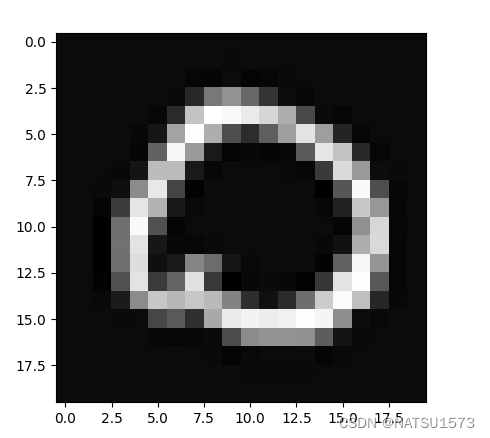
随机挑选一幅图像

# 预测
t = 100
img = x[t,1:]
plt.figure(1)
plt.imshow(img.reshape(20,20).T,cmap='gray')
plt.show()
num = predict(theta_all,x[t,:])
print(num)
# num=10