MATLAB quantreg 分数位回归 初步使用探究

打开 quantreg.m函数，在注释部分有以下说明：

% Quantile Regression
% 
% USAGE: [p,stats]=quantreg(x,y,tau[,order,nboot]);
% 
% INPUTS: 
%   x,y: data that is fitted. (x and y should be columns) ------------------------XY输入自变量因变量
%        Note: that if x is a matrix with several columns then multiple
%        linear regression is used and the "order" argument is not used.
%   tau: quantile used in regression.                      ------------------------分数位回归的参数τ
%   order: polynomial order. (default=1)------------------------------------------分数位回归多项式的阶数
%          (negative orders are interpreted as zero intercept)
%   nboot: number of bootstrap surrogates used in statistical inference.(default=200)-------bootstrap用于计算置信区间数目
%
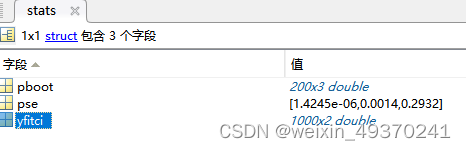
% stats is a structure with the following fields:
%      .pse:    standard error on p. (not independent)
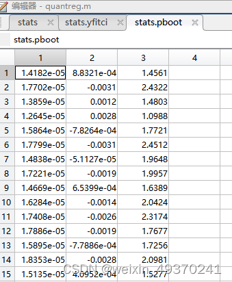
%      .pboot:  the bootstrapped polynomial coefficients.---
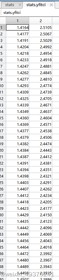
%      .yfitci: 95% confidence interval on "polyval(p,x)" or "x*p"---
%
% [If no output arguments are specified then the code will attempt to make a default test figure
% for convenience, which may not be appropriate for your data (especially if x is not sorted).]
%
% Note: uses bootstrap on residuals for statistical inference. (see help bootstrp)
% check also: http://www.econ.uiuc.edu/~roger/research/intro/rq.pdf
%

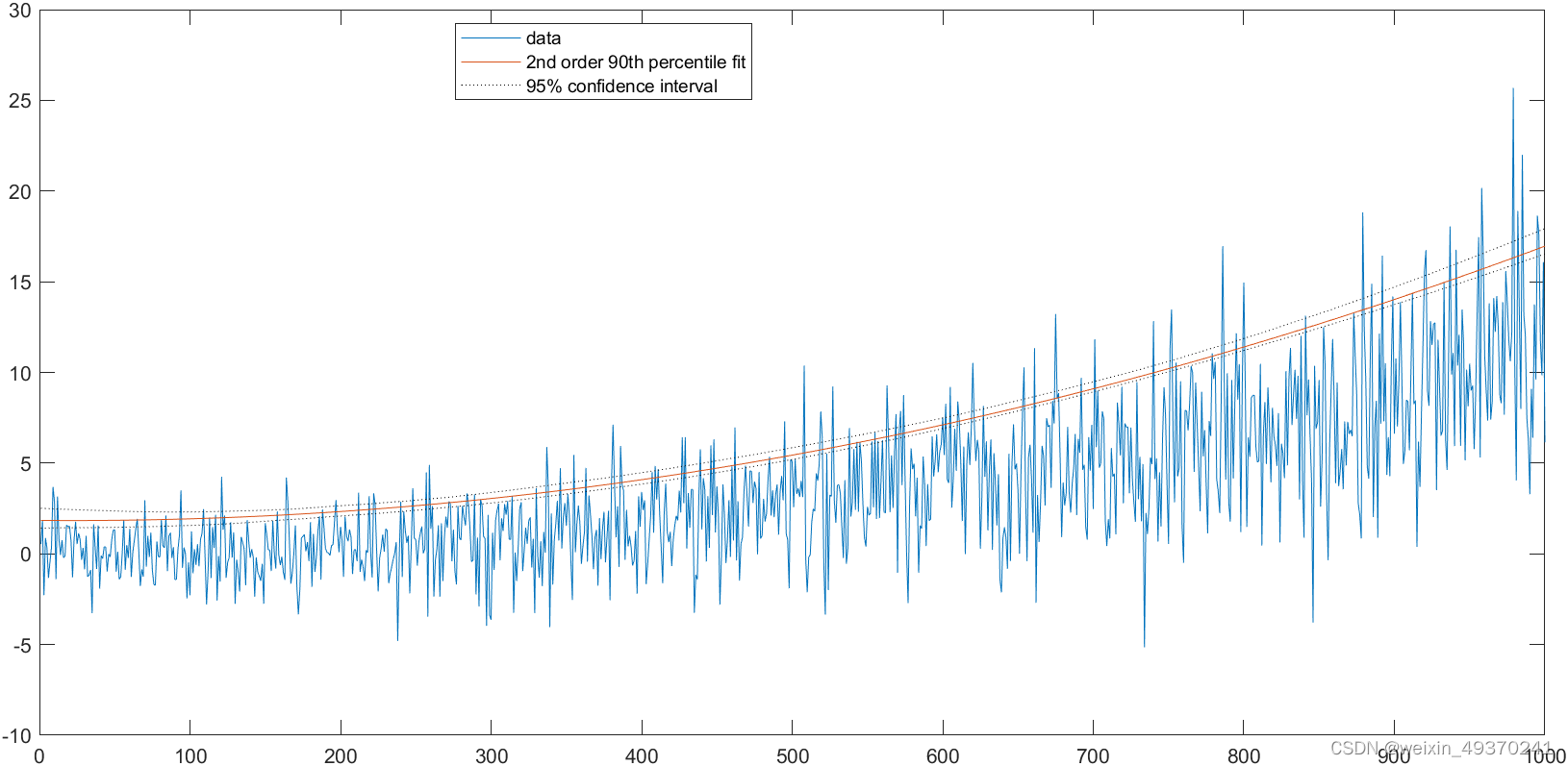
以下是 quantreg.m函数的一个官方示例：

输出变量stats是一个结构体，字段.yfitci是95%的置信区间【序列长度1000，置信区间为1000×2】，字段.pboot是每一次boot计算得出的多项式系数【在官方示例中，由于是二次函数拟合，每一次计算的结果的多项式系数有3个，y=ax2+bx+c，200次就有200×3的结果】。输出变量p是最终的唯一的多项式系数，用polyval(p,x)" or "x*p"来计算最终唯一的多项式曲线。

x=(1:1000)';
y=randn(size(x)).*(1+x/300)+(x/300).^2;
[p,stats]=quantreg(x,y,.9,2);
figure()
plot(x,y,x,polyval(p,x),x,stats.yfitci,'k:')
legend('data','2nd order 90th percentile fit','95% confidence interval','location','best')

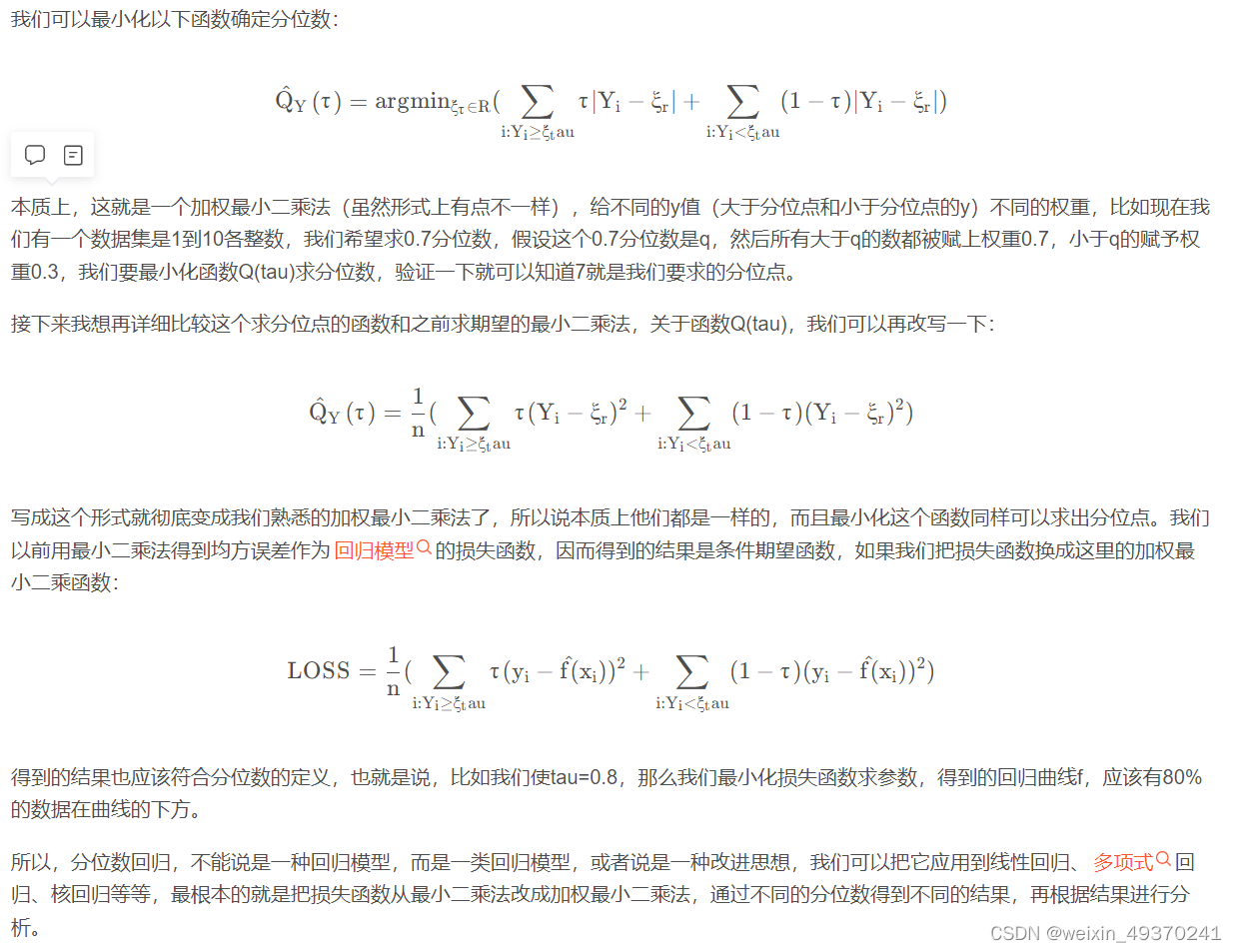
上图分别尝试了τ=0.9（红色） 0.1（绿色）和0.5（蓝色）的三种结果。τ的意义可参考这篇博客：【tau=0.8，那么我们最小化损失函数求参数，得到的回归曲线f，应该有80%的数据在曲线的下方。】
https://blog.csdn.net/jesseyule/article/details/95247155

x=(1:1000)';
y=randn(size(x)).*(1+x/300)+(x/300).^2;
[p,stats]=quantreg(x,y,.9,2);
figure()
plot(x,y,x,polyval(p,x),x,stats.yfitci,'k:')
legend('data','2nd order 90th percentile fit','95% confidence interval','location','best')

[p2,stats2]=quantreg(x,y,.1,2);
hold on
plot(x,polyval(p2,x),x,stats2.yfitci,'r:')
legend({'data','2nd order 90th percentile fit','95% confidence interval',...
    '2nd order 10th percentile fit','95% confidence interval'},'location','best')

[p3,stats3]=quantreg(x,y,.5,2);

figure()
plot(x,y,'k-','linewidth',2);hold on
plot(x,polyval(p,x),'r-','linewidth',2);
plot(x,stats.yfitci,'r--','linewidth',2);

plot(x,polyval(p2,x),'g-','linewidth',2);
plot(x,stats2.yfitci,'g--','linewidth',2);

plot(x,polyval(p3,x),'b-','linewidth',2);
plot(x,stats3.yfitci,'b--','linewidth',2);

legend({'data','2nd order 90th percentile fit','95%(90%) CI',...
    '2nd order 10th percentile fit','95%(10%) confidence interval',...
    '2nd order 50th percentile fit','95%(50%) confidence interval'},'location','best')

legend({'data','2nd order 90th percentile fit','95%(90%) confidence interval(down)','95%(90%) CI(up)'...
    '2nd order 10th percentile fit','95%(10%) CI(down)','95%(10%) CI(up)'...
    '2nd order 50th percentile fit','95%(50%) CI(down)','95%(50%) CI(up)'},...
    'location','best')