


本文将介绍DTW算法的目的和实现。其它参考:
离散序列的一致性度量方法:动态时间规整(DTW) http://blog.csdn.net/liyuefeilong/article/details/45748399
动态时间归整/规整/弯曲(Dynamic time warping,DTW) http://www.cnblogs.com/flypiggy/p/3603192.html
DTW相关维基百科戳这里
DTW是干什么的?
动态时间规整算法,就是把两个代表同一个类型的事物的不同长度序列进行时间上的“对齐”。比如DTW最常用的地方,语音识别中,同一个字母,由不同人发音,长短肯定不一样,把声音记录下来以后,它的信号肯定是很相似的,只是在时间上不太对整齐而已。所以我们需要用一个函数拉长或者缩短其中一个信号,使得它们之间的误差达到最小。
再来看看运动捕捉,比如当前有一个很快的拳击动作,另外有一个未加标签的动作,我想判断它是不是拳击动作,那么就要计算这个未加标签的动作和已知的拳击动作的相似度。但是呢,他们两个的动作长度不一样,比如一个是100帧,一个是200帧,那么这样直接对每一帧进行对比,计算到后面,误差肯定很大,那么我们把已知拳击动作的每一帧找到无标签的动作的对应帧中,使得它们的距离最短。这样便可以计算出两个运动的相似度,然后设定一个阈值,满足阈值范围就把未知动作加上“拳击”标签。
DTW怎么计算?
下面我们来总结一下DTW动态时间规整算法的简单的步骤:
1. 首先肯定是已知两个或者多个序列,但是都是两个两个的比较,所以我们假设有两个序列$A={a_1,a_2,a_3,...,a_m}$, $B={b_1,b_2,b_3,....,b_n}$,维度$m > n$2. 然后用欧式距离计算出每序列的每两点之间的距离,$D(a_i,b_j)$ 其中1≤i≤m,1≤j≤n
画出下表:

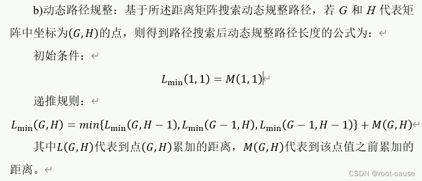
3. 接下来就是根据距离矩阵将最短路径找出来。从D(a1,a2)沿着某条路径到达D(am,bn)。找路径满足:假如当前节点是D(ai,bj),那么下一个节点必须是在D(i+1,j),D(i,j+1),D(i+1,j+1)之间选择,并且路径必须是最短的。计算的时候是按照动态规划的思想计算,也就是说在计算到达第(i,j)个节点的最短路径时候,考虑的是左上角也即第(i-1,j)、(i-1,j-1)、(i,j-1)这三个点到(i,j)的最短距离。
4. 接下来从最终的最短距离往回找到那条最佳的输出路径, 从D(a1,b1)到D(am,bn)。在这个路径上的所有距离的总和就是就是所需要的DTW距离
【注】如果不回溯路径,直接在第3步的时候将左上角三个节点到下一个节点最短的点作为最优路径节点,就是贪婪算法了。DTW是先计算起点到终点的最小值,然后从这个最小值回溯回去看看这个最小值都经过了哪些节点。
举个栗子:
已知:两个列向量a=[8 9 1]',b=[ 2 5 4 6]',其中'代表转置,也就是把行向量转换为列向量了
求:两个向量利用动态时间规整以后的最短距离
第一步:计算对应点的欧式距离矩阵d【注意开根号】
 6     3     4     2
 7     4     5     3
 1     4     3     5
第二步:计算累加距离D【从6出发到达5的累加距离】
 6     9    13    15
13    10    14    16
14    14    13    18
计算方法如下:
D(1,1)=d(1,1)=6
D(1,2)=D(1,1)+d(1,2)=9
...
D(2,2)=min(D(1,2),D(1,1),D(2,1))+d(2,2)=6+4=10
...
D(m,n)=min(D(m-1,n),D(m-1,n-1),D(m,n-1))+d(m,n)
网上有很多代码,但是大部分代码有误,比如网上流传比较多的错误版本:http://www.cnblogs.com/luxiaoxun/archive/2013/05/09/3069036.html
正确的代码可以自己写,挺简单,但是我找了一个可视化的代码,大家可以参考一下:
dtw.m
function [Dist,D,k,w,rw,tw]=dtw(r,t,pflag)
%
% [Dist,D,k,w,rw,tw]=dtw(r,t,pflag)
%
% Dynamic Time Warping Algorithm
% Dist is unnormalized distance between t and r
% D is the accumulated distance matrix
% k is the normalizing factor
% w is the optimal path
% t is the vector you are testing against
% r is the vector you are testing
% rw is the warped r vector
% tw is the warped t vector
% pflag  plot flag: 1 (yes), 0(no)
%
% Version comments:
% rw, tw and pflag added by Pau Mic

[row,M]=size(r); if (row > M) M=row; r=r'; end;
[row,N]=size(t); if (row > N) N=row; t=t'; end;
d=sqrt((repmat(r',1,N)-repmat(t,M,1)).^2); %this makes clear the above instruction Thanks Pau Mic
d
D=zeros(size(d));
D(1,1)=d(1,1);

for m=2:M
    D(m,1)=d(m,1)+D(m-1,1);
end
for n=2:N
    D(1,n)=d(1,n)+D(1,n-1);
end
for m=2:M
    for n=2:N
        D(m,n)=d(m,n)+min(D(m-1,n),min(D(m-1,n-1),D(m,n-1))); % this double MIn construction improves in 10-fold the Speed-up. Thanks Sven Mensing
    end
end

Dist=D(M,N);
n=N;
m=M;
k=1;
w=[M N];
while ((n+m)~=2)
    if (n-1)==0
        m=m-1;
    elseif (m-1)==0
        n=n-1;
    else
      [values,number]=min([D(m-1,n),D(m,n-1),D(m-1,n-1)]);
      switch number
      case 1
        m=m-1;
      case 2
        n=n-1;
      case 3
        m=m-1;
        n=n-1;
      end
  end
    k=k+1;
    w=[m n; w]; % this replace the above sentence. Thanks Pau Mic
end

% warped waves
rw=r(w(:,1));
tw=t(w(:,2));

%%%%%%%%%%%%%%%%%%%%%%%%%%%%%%%%%%%%%%%%%%%%%%%%%%%%%%%%%%%%%%%%%%%%%%%%%%%
if pflag

    % --- Accumulated distance matrix and optimal path
    figure('Name','DTW - Accumulated distance matrix and optimal path', 'NumberTitle','off');

    main1=subplot('position',[0.19 0.19 0.67 0.79]);
    image(D);
    cmap = contrast(D);
    colormap(cmap); % 'copper' 'bone', 'gray' imagesc(D);
    hold on;
    x=w(:,1); y=w(:,2);
    ind=find(x==1); x(ind)=1+0.2;
    ind=find(x==M); x(ind)=M-0.2;
    ind=find(y==1); y(ind)=1+0.2;
    ind=find(y==N); y(ind)=N-0.2;
    plot(y,x,'-w', 'LineWidth',1);
    hold off;
    axis([1 N 1 M]);
    set(main1, 'FontSize',7, 'XTickLabel','', 'YTickLabel','');

    colorb1=subplot('position',[0.88 0.19 0.05 0.79]);
    nticks=8;
    ticks=floor(1:(size(cmap,1)-1)/(nticks-1):size(cmap,1));
    mx=max(max(D));
    mn=min(min(D));
    ticklabels=floor(mn:(mx-mn)/(nticks-1):mx);
    colorbar(colorb1);
    set(colorb1, 'FontSize',7, 'YTick',ticks, 'YTickLabel',ticklabels);
    set(get(colorb1,'YLabel'), 'String','Distance', 'Rotation',-90, 'FontSize',7, 'VerticalAlignment','bottom');

    left1=subplot('position',[0.07 0.19 0.10 0.79]);
    plot(r,M:-1:1,'-b');
    set(left1, 'YTick',mod(M,10):10:M, 'YTickLabel',10*rem(M,10):-10:0)
    axis([min(r) 1.1*max(r) 1 M]);
    set(left1, 'FontSize',7);
    set(get(left1,'YLabel'), 'String','Samples', 'FontSize',7, 'Rotation',-90, 'VerticalAlignment','cap');
    set(get(left1,'XLabel'), 'String','Amp', 'FontSize',6, 'VerticalAlignment','cap');

    bottom1=subplot('position',[0.19 0.07 0.67 0.10]);
    plot(t,'-r');
    axis([1 N min(t) 1.1*max(t)]);
    set(bottom1, 'FontSize',7, 'YAxisLocation','right');
    set(get(bottom1,'XLabel'), 'String','Samples', 'FontSize',7, 'VerticalAlignment','middle');
    set(get(bottom1,'YLabel'), 'String','Amp', 'Rotation',-90, 'FontSize',6, 'VerticalAlignment','bottom');

    % --- Warped signals
    figure('Name','DTW - warped signals', 'NumberTitle','off');

    subplot(1,2,1);
    set(gca, 'FontSize',7);
    hold on;
    plot(r,'-bx');
    plot(t,':r.');
    hold off;
    axis([1 max(M,N) min(min(r),min(t)) 1.1*max(max(r),max(t))]);
    grid;
    legend('signal 1','signal 2');
    title('Original signals');
    xlabel('Samples');
    ylabel('Amplitude');

    subplot(1,2,2);
    set(gca, 'FontSize',7);
    hold on;
    plot(rw,'-bx');
    plot(tw,':r.');
    hold off;
    axis([1 k min(min([rw; tw])) 1.1*max(max([rw; tw]))]);
    grid;
    legend('signal 1','signal 2');
    title('Warped signals');
    xlabel('Samples');
    ylabel('Amplitude');
end
测试代码
test.m
clear
clc
a=[8 9 1 9 6 1 3 5]';
b=[2 5 4 6 7 8 3 7 7 2]';
[Dist,D,k,w,rw,tw] = DTW(a,b,1);
fprintf('最短距离为%d\n',Dist)
fprintf('最优路径为')
w
测试结果:
d =

     6     3     4     2     1     0     5     1     1     6
     7     4     5     3     2     1     6     2     2     7
     1     4     3     5     6     7     2     6     6     1
     7     4     5     3     2     1     6     2     2     7
     4     1     2     0     1     2     3     1     1     4
     1     4     3     5     6     7     2     6     6     1
     1     2     1     3     4     5     0     4     4     1
     3     0     1     1     2     3     2     2     2     3

最短距离为27
最优路径为
w =

     1     1
     1     2
     1     3
     1     4
     1     5
     1     6
     2     6
     3     7
     4     8
     5     9
     6    10
     7    10
     8    10
规整以后可视化如下


【更新日志:2019-9-11】
为了验证结果正确性,在python中也找到了一个工具库`dtw`
安装方法
pip install dtw
接收参数与返回参数
def dtw(x, y, dist, warp=1, w=inf, s=1.0):
    """
    Computes Dynamic Time Warping (DTW) of two sequences.
    :param array x: N1*M array
    :param array y: N2*M array
    :param func dist: distance used as cost measure
    :param int warp: how many shifts are computed.
    :param int w: window size limiting the maximal distance between indices of matched entries |i,j|.
    :param float s: weight applied on off-diagonal moves of the path. As s gets larger, the warping path is increasingly biased towards the diagonal
    Returns the minimum distance, the cost matrix, the accumulated cost matrix, and the wrap path.
    """
输入参数:前面x和y是输入的两个序列点,dist是计算距离的方法,因为有很多距离计算的方法,只不过通常使用欧式距离,直接使用numpy里面的linalg.norm即可。
返回值:这个d有点蒙,但是如果想得到上面的27那个结果,可以看accumulated cost matrix这个返回值,wrap path就是两条路径的对应点。
调用方法(官方案例):
import numpy as np

# We define two sequences x, y as numpy array
# where y is actually a sub-sequence from x
x = np.array([2, 0, 1, 1, 2, 4, 2, 1, 2, 0]).reshape(-1, 1)
y = np.array([1, 1, 2, 4, 2, 1, 2, 0]).reshape(-1, 1)

from dtw import dtw

euclidean_norm = lambda x, y: np.abs(x - y)
d, cost_matrix, acc_cost_matrix, path = dtw(x, y, dist=euclidean_norm)
print(d)
总结
DTW算法的计算复杂度是比较高的,如果数据量较大,使用DTW的matlab函数将会十分耗时,因为matlab的循环十分耗时。因此可以考虑用matlab调用DTW的C或C++函数,计算时间大大减少。例如我之前用过的一个数据,用DTW的matlab函数需要计算几十个小时,而调用DTW的C函数,只需要几十秒就能完成。我这里有之前已经配置好的C函数,效率很快。但是如果数据量较小,使用DTW的matlab函数也比较快。


 262
262

 被折叠的 条评论
为什么被折叠?
被折叠的 条评论
为什么被折叠?
 到【灌水乐园】发言


