YOLOv5-6.x源码分析（十）---- metrics.py

最新推荐文章于 2024-05-28 16:23:51 发布

JehanRio

最新推荐文章于 2024-05-28 16:23:51 发布

阅读量1.4k

点赞数 5

分类专栏： YOLOv5-6.x源码分析文章标签： YOLO 深度学习 python

本文链接：https://blog.csdn.net/weixin_51322383/article/details/130454335

版权

YOLOv5-6.x源码分析专栏收录该内容

11 篇文章 31 订阅

订阅专栏

文章目录

前言
🚀YOLOv5-6.x源码分析（十）---- metrics.py

前言

这个文件包含了各种目标检测的评价指标，包括计算mAP、混淆矩阵、IOU相关的函数，难度也非常的大，在看源码之前需要对这些定义有个了解。

导航：YOLOv5-6.x源码分析全流程记录

🚀YOLOv5-6.x源码分析（十）---- metrics.py

0. 导包

import math
import warnings
from pathlib import Path

import matplotlib.pyplot as plt
import numpy as np
import torch

基本就是些绘图、数学、矩阵相关的包

1. fitness

def fitness(x):
    w = [0.0, 0.0, 0.1, 0.9]  # weights for [P, R, mAP@0.5, mAP@0.5:0.95]
    # (torch.tensor).sum(1)
    return (x[:, :4] * w).sum(1)    # 每一行求和tensor为二维时返回一个以每一行求和为结果(常数)的行向量  1:行求和

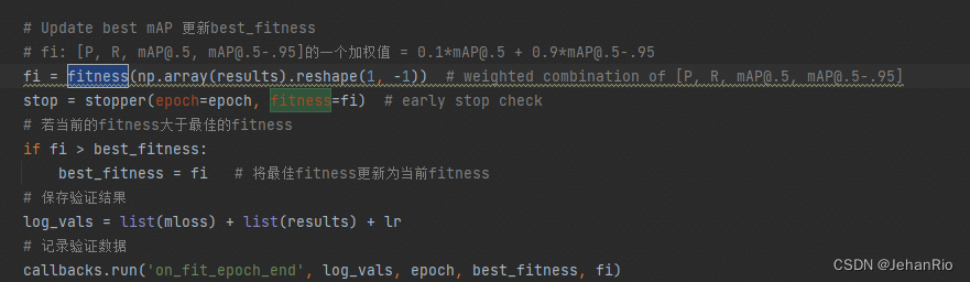
这个函数是通过指标加权的形式返回适应度(最终mAP)，判断模型好坏的指标不是mAP@0.5也不是mAP@0.5:0.95 而是[P, R, mAP@0.5, mAP@0.5:0.95]4者的加权。不过这里的P和R的权重都是0，相当于最终结果还是mAP的评价指标

该函数在train.py中的调用用来评价模型好坏

在这里插入图片描述

2. smooth

def smooth(y, f=0.05):
    # Box filter of fraction f
    nf = round(len(y) * f * 2) // 2 + 1  # number of filter elements (must be odd)
    p = np.ones(nf // 2)  # ones padding
    yp = np.concatenate((p * y[0], y, p * y[-1]), 0)  # y padded
    return np.convolve(yp, np.ones(nf) / nf, mode='valid')  # y-smoothed

用来计算预测框和真实框之间的差异的平滑值。具体来说，它通过将每个预测框的置信度与与其重叠度最高的真实框的重叠度进行加权平均来计算平滑值。这个平滑值可以用来评估模型的性能，例如，它可以用来计算模型在检测任务中的平均准确度和召回率等指标。在训练过程中，平滑值可以作为损失函数的一部分，帮助模型更好地学习预测框和真实框之间的差异。

3. ap_per_class

第一个难点来了，在看这个函数之前，建议先看一下这几篇文章。目标检测中的mAP是什么含义？

YOLO 模型的评估指标——IOU、Precision、Recall、F1-score、mAP

【python numpy】a.cumsum()、np.interp()、np.maximum.accumulate()、np.trapz()

计算mAP的方式：详解对象检测网络性能评价指标mAP计算

AP的定义就是PR取线与坐标轴围成的面积

具体计算步骤：

先找出每个类别的TP
将所有类别的TP按照conf降序排序
for 每一个类别
1. 计算这个类别的Recall和Precision
2. for 10个IOU阈值，计算mAP（调用compute_ap)函数

这里的FP = 1-TP

而TP的计算步骤为：

def ap_per_class(tp, conf, pred_cls, target_cls, plot=False, save_dir='.', names=(), eps=1e-16):
    """用于val.py中计算每个类的mAP
        计算每一个类的AP指标(average precision)还可以 绘制P-R曲线
        mAP基本概念: https://www.bilibili.com/video/BV1ez4y1X7g2
        Source: https://github.com/rafaelpadilla/Object-Detection-Metrics.
        :params tp(correct): [pred_sum, 10]=[1905, 10] bool 整个数据集所有图片中所有预测框在每一个iou条件下(0.5~0.95)10个是否是TP
        :params conf: [img_sum]=[1905] 整个数据集所有图片的所有预测框的conf
        :params pred_cls: [img_sum]=[1905] 整个数据集所有图片的所有预测框的类别
                这里的tp、conf、pred_cls是一一对应的
        :params target_cls: [gt_sum]=[929] 整个数据集所有图片的所有gt框的class
        :params plot: bool
        :params save_dir: runs\train\exp30
        :params names: dict{key(class_index):value(class_name)} 获取数据集所有类别的index和对应类名
        :return p[:, i]: [nc] 最大平均f1时每个类别的precision
        :return r[:, i]: [nc] 最大平均f1时每个类别的recall
        :return ap: [71, 10] 数据集每个类别在10个iou阈值下的mAP
        :return f1[:, i]: [nc] 最大平均f1时每个类别的f1
        :return unique_classes.astype('int32'): [nc] 返回数据集中所有的类别index
        """
    # 计算mAP 需要将tp按照conf降序排列
    # Sort by objectness  按conf从大到小排序 返回数据对应的索引
    i = np.argsort(-conf)
    # 得到重新排序后对应的 tp, conf, pre_cls
    tp, conf, pred_cls = tp[i], conf[i], pred_cls[i]

    # Find unique classes  对类别去重, 因为计算ap是对每类进行
    unique_classes, nt = np.unique(target_cls, return_counts=True)  # 去除其中重复的元素，并按元素由大到小返回一个新的无元素重复的元组或者列表
    # px: [0, 1] 中间间隔1000个点 x坐标(用于绘制P-Conf、R-Conf、F1-Conf)
    # py: y坐标[] 用于绘制IOU=0.5时的PR曲线
    nc = unique_classes.shape[0]  # 数据集类别数 number of classes, number of detections nc:71

    # Create Precision-Recall curve and compute AP for each class
    px, py = np.linspace(0, 1, 1000), []  # for plotting 绘图
    ap, p, r = np.zeros((nc, tp.shape[1])), np.zeros((nc, 1000)), np.zeros((nc, 1000))
    for ci, c in enumerate(unique_classes):
        # i: 记录着所有预测框是否是c类别框   是c类对应位置为True, 否则为False
        i = pred_cls == c
        # n_l: gt框中的c类别框数量  = tp+fn   254
        n_l = nt[ci]  # number of labels
        # n_p: 预测框中c类别的框数量   695
        n_p = i.sum()  # number of predictions
        if n_p == 0 or n_l == 0:
            continue

        # Accumulate FPs and TPs
        fpc = (1 - tp[i]).cumsum(0) # 沿着指定轴的元素累加和所组成的数组，其形状应与输入数组a一致
        tpc = tp[i].cumsum(0)   # fp[i] = 1 - tp[i]

        # Recall=TP/(TP+FN)  加一个1e-16的目的是防止分母为0
        # n_l=TP+FN=num_gt: c类的gt个数=预测是c类而且预测正确+预测不是c类但是预测错误
        # recall: 类别为c 顺序按置信度排列 截至每一个预测框的各个iou阈值下的召回率
        recall = tpc / (n_l + eps)  # recall curve
        # 返回所有类别, 横坐标为conf(值为px=[0, 1, 1000] 0~1 1000个点)对应的recall值  r=[nc, 1000]  每一行从小到大
        # np.interp：这是一个线性插值函数
        r[ci] = np.interp(-px, -conf[i], recall[:, 0], left=0)  # negative x, xp because xp decreases

        # Precision=TP/(TP+FP)
        # precision: 类别为c 顺序按置信度排列 截至每一个预测框的各个iou阈值下的精确率
        precision = tpc / (tpc + fpc)  # precision curve
        # 返回所有类别, 横坐标为conf(值为px=[0, 1, 1000] 0~1 1000个点)对应的precision值  p=[nc, 1000]
        # 总体上是从小到大 但是细节上有点起伏 如: 0.91503 0.91558 0.90968 0.91026 0.90446 0.90506
        p[ci] = np.interp(-px, -conf[i], precision[:, 0], left=1)  # p at pr_score

        # AP from recall-precision curve
        # 这里执行10次计算ci这个类别在所有mAP阈值下的平均mAP  ap[nc, 10]
        for j in range(tp.shape[1]):
            ap[ci, j], mpre, mrec = compute_ap(recall[:, j], precision[:, j])
            if plot and j == 0:
                py.append(np.interp(px, mrec, mpre))  # precision at mAP@0.5

    # Compute F1 (harmonic mean of precision and recall)
    # 计算F1分数 P和R的调和平均值  综合评价指标
    f1 = 2 * p * r / (p + r + eps)
    names = [v for k, v in names.items() if k in unique_classes]  # list: only classes that have data
    names = dict(enumerate(names))  # to dict
    if plot:
        plot_pr_curve(px, py, ap, Path(save_dir) / 'PR_curve.png', names)   # pr图
        plot_mc_curve(px, f1, Path(save_dir) / 'F1_curve.png', names, ylabel='F1')  # f1
        plot_mc_curve(px, p, Path(save_dir) / 'P_curve.png', names, ylabel='Precision') # P_conf
        plot_mc_curve(px, r, Path(save_dir) / 'R_curve.png', names, ylabel='Recall')    # R_conf

    i = smooth(f1.mean(0), 0.1).argmax()  # max F1 index
    p, r, f1 = p[:, i], r[:, i], f1[:, i]
    tp = (r * nt).round()  # true positives
    fp = (tp / (p + eps) - tp).round()  # false positives
    return tp, fp, p, r, f1, ap, unique_classes.astype(int)

这个函数会在val.py中用到，用于绘制各种曲线

4. compute_ap

def compute_ap(recall, precision):
    """ Compute the average precision, given the recall and precision curves
    # Arguments
        recall:    The recall curve (list)
        precision: The precision curve (list)
    # Returns
        Average precision, precision curve, recall curve
    """

    # 在开头和末尾添加保护值 防止全零的情况出现 value Append sentinel values to beginning and end
    mrec = np.concatenate(([0.0], recall, [1.0]))
    mpre = np.concatenate(([1.0], precision, [0.0]))

    # Compute the precision envelope
    '''
        np.maximum.accumulate:计算数组（或数组的特定轴）的累积最大值
        保证mpre是从大到小单调的(左右可以相同)
        eg:
            d = np.array([2, 0, 3, -4, -2, 7, 9])
            c = np.maximum.accumulate(d)
            print(c)   # array([2, 2, 3, 3, 3, 7, 9])
        这样可能是为了更好计算mAP 因为如果一直起起伏伏太难算了(x间隔很小就是一个矩形) 而且这样做误差也不会很大 两个之间的数都是间隔很小的
    '''

    mpre = np.flip(np.maximum.accumulate(np.flip(mpre)))    # np.flip翻转顺序

    # Integrate area under curve
    method = 'interp'  # methods: 'continuous', 'interp'
    if method == 'interp':  # 用一些典型的间断点来计算AP
        x = np.linspace(0, 1, 101)  # 101-point interp (COCO)
        ap = np.trapz(np.interp(x, mrec, mpre), x)  # integrate 计算两个list对应点与点之间四边形的面积 以定积分形式估算AP 第一个参数是y 第二个参数是x
    else:  # 'continuous'
        # 通过错位的方式 判断哪个点当前位置到下一个位置值发生改变 并通过！=判断 返回一个布尔数组
        i = np.where(mrec[1:] != mrec[:-1])[0]  # points where x axis (recall) changes
        # 值改变了就求出当前矩阵的面积  值没变就说明当前矩阵和下一个矩阵的高相等所有可以合并计算
        ap = np.sum((mrec[i + 1] - mrec[i]) * mpre[i + 1])  # area under curve

    return ap, mpre, mrec

这个函数就是计算某个类别在某个IOU下的mAP，会在上面的函数中用到。

参数：

precision: (list) [1635] 在某个iou阈值下某个类别所有的预测框的precision
总体上是从大到小但是细节上有点起伏如: 0.91503 0.91558 0.90968 0.91026 0.90446 0.90506(每个预测框的precision都是截至到这个预测框为止的总precision)
recall:(list) [1635] 在某个iou阈值下某个类别所有的预测框的recall 从小到大 (每个预测框的recall都是截至到这个预测框为止的总recall)

返回值：

ap: Average precision 返回某类别在某个iou下的mAP(均值) [1]
mpre: precision curve [1637] 返回开头 + 输入precision(排序后) + 末尾
mrec: recall curve [1637] 返回开头 + 输入recall + 末尾

5. ConfusionMatrix

class ConfusionMatrix:
    # Updated version of https://github.com/kaanakan/object_detection_confusion_matrix
    # 类别、预测框置信度阈值、iou阈值
    def __init__(self, nc, conf=0.25, iou_thres=0.45):
        # 背景也算一类
        # 如果某个gt[j]没用任何pred正样本匹配到 那么[nc, gt[j]_class] += 1
        # 如果某个pred[i]负样本且没有哪个gt与之对应 那么[pred[i]_class nc] += 1
        self.matrix = np.zeros((nc + 1, nc + 1))
        self.nc = nc  # number of classes
        self.conf = conf
        self.iou_thres = iou_thres

    def process_batch(self, detections, labels):
        """
        :params detections: [N, 6] = [pred_obj_num, x1y1x2y2+object_conf+cls] = [300, 6]
                            一个batch中一张图的预测信息  其中x1y1x2y2是映射到原图img的
        :params labels: [M, 5] = [gt_num, class+x1y1x2y2] = [17, 5] 其中x1y1x2y2是映射到原图img的
        :return: None, updates confusion matrix accordingly
        """
        # [10, 6] 筛除置信度过低的预测框(和nms差不多)
        if detections is None:
            gt_classes = labels.int()
            for i, gc in enumerate(gt_classes):
                self.matrix[self.nc, gc] += 1  # background FN
            return

        detections = detections[detections[:, 4] > self.conf]
        gt_classes = labels[:, 0].int()
        detection_classes = detections[:, 5].int()
        # 求出所有gt框和所有pred框的iou [17, x1y1x2y2] + [10, x1y1x2y2] => [17, 10] [i, j] 第i个gt框和第j个pred的iou
        iou = box_iou(labels[:, 1:], detections[:, :4])

        x = torch.where(iou > self.iou_thres)
        if x[0].shape[0]:
            # 1、matches: [10, gt_index+pred_index+iou] = [10, 3]
            matches = torch.cat((torch.stack(x, 1), iou[x[0], x[1]][:, None]), 1).cpu().numpy()
            if x[0].shape[0] > 1:
                # 2、matches按第三列iou从大到小重排序
                matches = matches[matches[:, 2].argsort()[::-1]]
                # 3、取第二列中各个框首次出现(不同预测的框)的行(即每一种预测的框中iou最大的那个)
                matches = matches[np.unique(matches[:, 1], return_index=True)[1]]
                # 4、matches再按第三列iou从大到小重排序
                matches = matches[matches[:, 2].argsort()[::-1]]
                # 5、取第一列中各个框首次出现(不同gt的框)的行(即每一种gt框中iou最大的那个)
                matches = matches[np.unique(matches[:, 0], return_index=True)[1]]
                # 经过这样的处理 最终得到每一种预测框与所有gt框中iou最大的那个(在大于阈值的前提下)
                # 预测框唯一  gt框也唯一  这样得到的matches对应的Pred都是正样本Positive
        else:
            matches = np.zeros((0, 3))

        n = matches.shape[0] > 0
        m0, m1, _ = matches.transpose().astype(int)
        for i, gc in enumerate(gt_classes):
            j = m0 == i
            if n and sum(j) == 1:
                self.matrix[detection_classes[m1[j]], gc] += 1  # correct
            else:
                self.matrix[self.nc, gc] += 1  # background FP

        if n:
            for i, dc in enumerate(detection_classes):
                if not any(m1 == i):
                    self.matrix[dc, self.nc] += 1  # background FN

    def matrix(self):
        return self.matrix

    # 移除背景
    def tp_fp(self):
        tp = self.matrix.diagonal()  # true positives
        fp = self.matrix.sum(1) - tp  # false positives
        # fn = self.matrix.sum(0) - tp  # false negatives (missed detections)
        return tp[:-1], fp[:-1]  # remove background class

    def plot(self, normalize=True, save_dir='', names=()):
        """
        :params normalize: 是否将混淆矩阵归一化 默认True
        :params save_dir: runs/train/expn 混淆矩阵保存地址
        :params names: 数据集的所有类别名
        :return None
        """
        try:
            import seaborn as sn

            array = self.matrix / ((self.matrix.sum(0).reshape(1, -1) + 1E-9) if normalize else 1)  # normalize columns
            array[array < 0.005] = np.nan  # don't annotate (would appear as 0.00)

            fig = plt.figure(figsize=(12, 9), tight_layout=True)
            nc, nn = self.nc, len(names)  # number of classes, names
            sn.set(font_scale=1.0 if nc < 50 else 0.8)  # for label size
            labels = (0 < nn < 99) and (nn == nc)  # apply names to ticklabels
            # 绘制热力图 即混淆矩阵可视化
            with warnings.catch_warnings():
                warnings.simplefilter('ignore')  # suppress empty matrix RuntimeWarning: All-NaN slice encountered
                # sean.heatmap: 热力图  data: 数据矩阵  annot: 为True时为每个单元格写入数据值 False用颜色深浅表示
                # annot_kws: 格子外框宽度  fmt: 添加注释时要使用的字符串格式代码 cmap: 指色彩颜色的选择
                # square: 是否是正方形  xticklabels、yticklabels: xy标签
                sn.heatmap(array,
                           annot=nc < 30,
                           annot_kws={
                               "size": 8},
                           cmap='Blues',
                           fmt='.2f',
                           square=True,
                           vmin=0.0,
                           xticklabels=names + ['background FP'] if labels else "auto",
                           yticklabels=names + ['background FN'] if labels else "auto").set_facecolor((1, 1, 1))
            fig.axes[0].set_xlabel('True')
            fig.axes[0].set_ylabel('Predicted')
            fig.savefig(Path(save_dir) / 'confusion_matrix.png', dpi=250)
            plt.close()
        except Exception as e:
            print(f'WARNING: ConfusionMatrix plot failure: {e}')

    def print(self):
        for i in range(self.nc + 1):
            print(' '.join(map(str, self.matrix[i])))

没看懂。。。

看这段代码应该是需要debug的，不然完全不知道在干嘛，五一假期的我效率太低了，只想偷懒完成任务，后面再补吧。。。

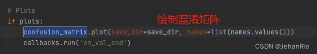
这个类会在val.py中调用，用于画出混淆矩阵

在这里插入图片描述

6. bbox_iou

def bbox_iou(box1, box2, xywh=True, GIoU=False, DIoU=False, CIoU=False, eps=1e-7):
    # Returns Intersection over Union (IoU) of box1(1,4) to box2(n,4)

    # Get the coordinates of bounding boxes
    if xywh:  # transform from xywh to xyxy
        (x1, y1, w1, h1), (x2, y2, w2, h2) = box1.chunk(4, 1), box2.chunk(4, 1) # 分割成chunk_num个tensor块,返回一个元组
        w1_, h1_, w2_, h2_ = w1 / 2, h1 / 2, w2 / 2, h2 / 2
        b1_x1, b1_x2, b1_y1, b1_y2 = x1 - w1_, x1 + w1_, y1 - h1_, y1 + h1_
        b2_x1, b2_x2, b2_y1, b2_y2 = x2 - w2_, x2 + w2_, y2 - h2_, y2 + h2_
    else:  # x1, y1, x2, y2 = box1
        b1_x1, b1_y1, b1_x2, b1_y2 = box1.chunk(4, 1)
        b2_x1, b2_y1, b2_x2, b2_y2 = box2.chunk(4, 1)
        w1, h1 = b1_x2 - b1_x1, b1_y2 - b1_y1
        w2, h2 = b2_x2 - b2_x1, b2_y2 - b2_y1

    # Intersection area
    inter = (torch.min(b1_x2, b2_x2) - torch.max(b1_x1, b2_x1)).clamp(0) * \
            (torch.min(b1_y2, b2_y2) - torch.max(b1_y1, b2_y1)).clamp(0)

    # Union Area
    union = w1 * h1 + w2 * h2 - inter + eps

    # IoU
    iou = inter / union
    if CIoU or DIoU or GIoU:
        # 两个框的最小闭包区域的width
        cw = torch.max(b1_x2, b2_x2) - torch.min(b1_x1, b2_x1)  # convex (smallest enclosing box) width
        # 两个框的最小闭包区域的height
        ch = torch.max(b1_y2, b2_y2) - torch.min(b1_y1, b2_y1)  # convex height
        if CIoU or DIoU:  # Distance or Complete IoU https://arxiv.org/abs/1911.08287v1
            c2 = cw ** 2 + ch ** 2 + eps  # convex diagonal squared
            rho2 = ((b2_x1 + b2_x2 - b1_x1 - b1_x2) ** 2 + (b2_y1 + b2_y2 - b1_y1 - b1_y2) ** 2) / 4  # center dist ** 2
            if CIoU:  # https://github.com/Zzh-tju/DIoU-SSD-pytorch/blob/master/utils/box/box_utils.py#L47
                v = (4 / math.pi ** 2) * torch.pow(torch.atan(w2 / (h2 + eps)) - torch.atan(w1 / (h1 + eps)), 2)
                with torch.no_grad():
                    alpha = v / (v - iou + (1 + eps))
                return iou - (rho2 / c2 + v * alpha)  # CIoU
            return iou - rho2 / c2  # DIoU
        c_area = cw * ch + eps  # convex area
        return iou - (c_area - union) / c_area  # GIoU https://arxiv.org/pdf/1902.09630.pdf
    return iou  # IoU

这个函数是用来计算矩阵框间的IOU的，现在有很多种iou变种，如：iou/Giou/Diou/Ciou。

这个函数通常用来在ComputeLoss中计算回归损失（bbox损失）

7. plot_pr_curve

def plot_pr_curve(px, py, ap, save_dir=Path('pr_curve.png'), names=()):
    """用于ap_per_class函数
        Precision-recall curve  绘制PR曲线
        :params px: [1000] 横坐标 recall 值为0~1直接取1000个数
        :params py: list{nc} nc个[1000] 所有类别在IOU=0.5,横坐标为px(recall)时的precision
        :params ap: [nc, 10] 所有类别在每个IOU阈值下的平均mAP
        :params save_dir: runs\test\exp54\PR_curve.png  PR曲线存储位置
        :params names: {dict:80} 数据集所有类别的字典 key:value
        """
    # Precision-recall curve
    fig, ax = plt.subplots(1, 1, figsize=(9, 6), tight_layout=True)
    py = np.stack(py, axis=1)

    # 画出所有类别在10个IOU阈值下的PR曲线
    if 0 < len(names) < 21:  # 如果<21 classes就一个个类画 因为要显示图例就必须一个个画
        for i, y in enumerate(py.T):
            ax.plot(px, y, linewidth=1, label=f'{names[i]} {ap[i, 0]:.3f}')  # plot(recall, precision)
    else:   # 如果>=21 classes 显示图例就会很乱 所以就不显示图例了 可以直接输入数组 x[1000] y[1000, 71]
        ax.plot(px, py, linewidth=1, color='grey')  # plot(recall, precision)

    ax.plot(px, py.mean(1), linewidth=3, color='blue', label='all classes %.3f mAP@0.5' % ap[:, 0].mean())
    ax.set_xlabel('Recall')
    ax.set_ylabel('Precision')
    ax.set_xlim(0, 1)
    ax.set_ylim(0, 1)
    plt.legend(bbox_to_anchor=(1.04, 1), loc="upper left")
    fig.savefig(save_dir, dpi=250)
    plt.close()

这个函数用于绘制PR取线，会在ap_per_class中调用

8. plot_mc_curve

def plot_mc_curve(px, py, save_dir=Path('mc_curve.png'), names=(), xlabel='Confidence', ylabel='Metric'):
    """用于ap_per_class函数
        Metric-Confidence curve 可用于绘制 F1-Confidence/P-Confidence/R-Confidence曲线
        :params px: [0, 1, 1000] 横坐标 0-1 1000个点 conf   [1000]
        :params py: 对每个类, 针对横坐标为conf=[0, 1, 1000] 对应的f1/p/r值 纵坐标 [71, 1000]
        :params save_dir: 图片保存地址
        :parmas names: 数据集names
        :params xlabel: x轴标签
        :params ylabel: y轴标签
        """
    # Metric-confidence curve
    fig, ax = plt.subplots(1, 1, figsize=(9, 6), tight_layout=True)

    # 画出所有类别的F1-Confidence/P-Confidence/R-Confidence曲线
    if 0 < len(names) < 21:  # display per-class legend if < 21 classes
        for i, y in enumerate(py):
            ax.plot(px, y, linewidth=1, label=f'{names[i]}')  # plot(confidence, metric)
    else:
        ax.plot(px, py.T, linewidth=1, color='grey')  # plot(confidence, metric)

    y = smooth(py.mean(0), 0.05)
    ax.plot(px, y, linewidth=3, color='blue', label=f'all classes {y.max():.2f} at {px[y.argmax()]:.3f}')
    ax.set_xlabel(xlabel)
    ax.set_ylabel(ylabel)
    ax.set_xlim(0, 1)
    ax.set_ylim(0, 1)
    plt.legend(bbox_to_anchor=(1.04, 1), loc="upper left")
    fig.savefig(save_dir, dpi=250)
    plt.close()

绘制F1取线，F1-score就是用来用来权衡Precision和Recall的平均值。

根据F1-score的定义式可知，F1-score也是取平均值，只不过强调的是二者之间的较小值。通过F1-score的方式来权衡Precision与Recall，可以有效的避免短板效应，这在数学上被称为调和平均数。

总结

这个脚本的代码量不多，但是每一个函数都非常的复杂，这个脚本要和val.py一起看，纵观整个专栏，我掌握的最不透彻的就是这个文件和val.py了，很多函数也只是了解它的作用，并没有看懂它的源码。

有时候我经常在想，有必要看那么细吗？这对我有什么帮助吗？包括我也问了我的老师和学长，有必要去挖YOLOv5的源码吗，老师也说没有必要。但是对于我来说，我是在这方面喜欢刨根问底的人，尽管我用了这么久的YOLOv5，但我总对他的很多执行过程云里雾里，让我去挖一遍源码，真的能解决我很多的疑惑。比如我之前一直没搞清bbox损失和置信度损失之间的关系，经过这次的学习后，让我大彻大悟。

这段时间看了很多博主的源码剖析，不得不说，他们做的都非常的好，讲的也非常的通透，而我许多地方看不懂仍然还是写了上去，算是为了给这个博客专栏做得更加完善吧，所以如果你看到我的很多地方讲的不透彻，你可以再看看我最下方References，或者去搜搜别的博主，肯定能解决你的疑惑。当然，我也非常欢迎你能和我进行讨论。如果你也能像我一样去写一个属于你自己的专栏解析，那我觉得这件事情。。。泰裤辣！！！

JehanRio

关注

5
点赞
踩
13

收藏

觉得还不错? 一键收藏
4
评论
YOLOv5-6.x源码分析（十）---- metrics.py

这个文件包含了各种目标检测的评价指标，包括计算mAP、混淆矩阵、IOU相关的函数，难度也非常的大，在看源码之前需要对这些定义有个了解。导航YOLOv5-6.x源码分析全流程记录这个脚本的代码量不多，但是每一个函数都非常的复杂，这个脚本要和val.py一起看，纵观整个专栏，我掌握的最不透彻的就是这个文件和val.py了，很多函数也只是了解它的作用，并没有看懂它的源码。有时候我经常在想，有必要看那么细吗？这对我有什么帮助吗？包括我也问了我的老师和学长，有必要去挖YOLOv5的源码吗，老师也说没有必要。
复制链接

扫一扫