机器翻译：引入注意力机制的Encoder-Decoder深度神经网络训练实战中英文互译（完结篇）

---

前言

注意力机制是一种在深度学习中广泛使用的技术，它可以有效地处理输入序列和输出序列之间的对应关系。其中，Encoder-Decoder是一种常见的注意力机制，它主要用于序列到序列的任务，例如机器翻译、语音识别等。在Encoder-Decoder中，输入序列首先通过一个编码器进行编码，然后再通过一个解码器进行解码，最终生成输出序列。在这个过程中，注意力机制可以帮助模型更好地理解输入序列中的重要信息，并在生成输出序列的过程中更加准确地对其进行利用。由于其出色的性能和广泛的适用性，注意力机制的Encoder-Decoder已经成为自然语言处理和语音识别等领域中的重要技术之一。

---

要做一个中英互译的神经网络训练，我们需要有：
预：可供训练的数据集 数据集我已经上传数据集（免费）
1.数据的预处理
2.模型配置
3.模型训练
整个过程是在kaggle上进行的

一、数据的预处理

数据的预处理和有关数据集的简介，我上篇文章已经讲解，有需要的直接可以查阅机器翻译 深度学习预处理实战（中英文互译）一
在这里我直接附上代码：

import tensorflow as tf
import matplotlib.pyplot as plt
import matplotlib.ticker as ticker
from sklearn.model_selection import train_test_split
import unicodedata
import re
import numpy as np
import os
import io
import time
import pandas as pd
import numpy as np
import jieba
jieba.initialize() # 手动初始化jieba资源，提高分词效率。
jieba.enable_paddle() # 启动paddle模式。 0.40版之后开始支持，早期版本不支持

# 判断是否包含中文
def is_chinese(string):
  """
  检查整个字符串是否包含中文
  :param string: 需要检查的字符串
  :return: bool
  """
  for ch in string:
    if u'\u4e00' <= ch <= u'\u9fa5':
      return True
  return False

# 中英文预处理
def preprocess_sentence(w):
  if not is_chinese(w):
    w = w.lower()

    # 除了 (a-z, A-Z, ".", "?", "!", ",")，将所有字符替换为空格
    w = re.sub(r"[^a-zA-Z?.!,]+", " ", w)
    w = w.rstrip().strip()

    # 给句子加上开始和结束标记，以便模型知道每个句子开始和结束的位置
    w = '<start> ' + w + ' <end>'
  else:
    w = re.sub(r"[^\u4e00-\u9fa5，。？！]+", "", w)
    w = w.strip()
    # seg_list = jieba.cut(w,use_paddle=True) # 使用paddle模式分词
    # w= ' '.join(list(seg_list))
    w = 分字(w)
    # 给句子加上开始和结束标记，以便模型知道每个句子开始和结束的位置
    w = '<start> ' + w + ' <end>'
  return w

def 分字(str):
  line = str.strip()
  pattern = re.compile('[^\u4e00-\u9fa5，。？！]')
  en = ' '.join(pattern.split(line)).strip()
  result=''
  for character in en:
    result+=character+' '
  return result.strip()

# 调用预处理方法，并返回这样格式的句子对：[english, chinese]
def create_dataset(path, num_examples):
  lines = io.open(path, encoding='UTF-8').read().strip().split('\n')
  word_pairs = [[preprocess_sentence(w) for w in l.split('\t')[0:2][::-1]] for l in lines[:num_examples]]
  return zip(*word_pairs)

# 判断词序列长度
def max_length(tensor):
  return max(len(t) for t in tensor)

# 词符化
def tokenize(lang):
  lang_tokenizer = tf.keras.preprocessing.text.Tokenizer(filters='')
  lang_tokenizer.fit_on_texts(lang)
  tensor = lang_tokenizer.texts_to_sequences(lang)
  tensor = tf.keras.preprocessing.sequence.pad_sequences(tensor,padding='post')
  return tensor, lang_tokenizer

# 创建清理过的输入输出对
def load_dataset(path, num_examples=None):
  chs, en = create_dataset(path, num_examples)
  input_tensor, inp_lang_tokenizer = tokenize(en)
  target_tensor, targ_lang_tokenizer = tokenize(chs)
  return input_tensor, target_tensor, inp_lang_tokenizer, targ_lang_tokenizer

# 格式化显示字典内容
def convert(lang, tensor):
  for t in tensor:
    if t!=0:
      print("%d ----> %s" % (t, lang.index_word[t]))

if __name__=="__main__":
  num_examples = 100
  # 读取英中互译文件
  path_to_file = '/kaggle/input/tansantcmn/cmn.txt'
  input_tensor, target_tensor, inp_lang_tokenizer, targ_lang_tokenizer = load_dataset(path_to_file, num_examples)

  # 计算最大长度
  max_length_input, max_length_target = max_length(input_tensor), max_length(target_tensor)

  # 将数据集拆分为训练和验证集
  input_tensor_train, input_tensor_val, target_tensor_train, target_tensor_val = train_test_split(input_tensor, target_tensor, test_size=0.2)

  # 显示长度
  print("Max length of input:", max_length_input)
  print("Max length of target:", max_length_target)

  # 显示词典长度
  print("Input vocabulary size:", len(inp_lang_tokenizer.word_index))
  print("Target vocabulary size:", len(targ_lang_tokenizer.word_index))

  # 显示样例
  print("Example input sequence:")
  convert(inp_lang_tokenizer, input_tensor_train[0])
  print("Actual input sentence:")
  print(' '.join([inp_lang_tokenizer.index_word[i] for i in input_tensor_train[0] if i not in [0]]))
  print("\nExample target sequence:")
  convert(targ_lang_tokenizer, target_tensor_train[0])
  print("Actual target sentence:")
  print(' '.join([targ_lang_tokenizer.index_word[i] for i in target_tensor_train[0] if i not in [0]]))
print(len(input_tensor_train), len(target_tensor_train), len(input_tensor_val), len(target_tensor_val))

# 显示编码后的源语言（中文）张量数据集示例
print('经过编码后的源语言（中文）张量数据集示例：')
print(input_tensor[:3])

先看运行结果

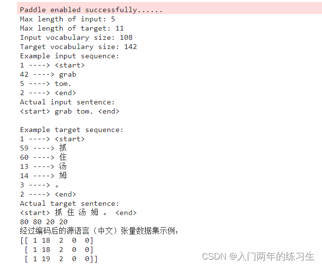
我们从数据集中随机抽取了一句话来进行翻译（grab tom.),可以看到翻译的结果（抓住汤姆）。此时效果还是不错的
我们这里是英译中的翻译，如果小伙伴想进行中译英，可以在（# 中英文预处理）函数中将not is_chinese(w):中的not去掉。
接下来我们来尝试使用注意力机制来进行深度学习训练

二、模型配置

要进行深度学习的训练，我们首先需要搭建模型
实现了一个基于注意力机制的Encoder-Decoder模型，
这里主要分为三个部分：
Encoder、
BahdanauAttention
Decoder。

Encoder部分
Encoder是一个继承自tf.keras.Model的类，用于对输入序列进行编码。其中，输入序列通过Embedding层进行嵌入后，再通过GRU层进行编码，最终输出编码器的编码结果和隐藏状态。

class Encoder(tf.keras.Model):
    def __init__(self, vocab_size, embedding_dim, enc_units, batch_sz):
        super(Encoder, self).__init__()
        self.batch_sz = batch_sz
        self.enc_units = enc_units
        self.embedding = tf.keras.layers.Embedding(vocab_size, embedding_dim)
        self.gru = tf.keras.layers.GRU(self.enc_units,return_sequences=True,return_state=True,recurrent_initializer='glorot_uniform')
    def call(self, x, hidden):
        x = self.embedding(x)
        output, state = self.gru(x, initial_state = hidden)
        return output, state
    def initialize_hidden_state(self):
        return tf.zeros((self.batch_sz, self.enc_units))

BahdanauAttention
BahdanauAttention是一个继承自tf.keras.layers.Layer的类，用于计算注意力向量和注意力权重。其中，通过Dense层将解码器的隐状态和编码器的编码结果映射到同一维度，然后通过tanh函数和Dense层计算分数，再通过softmax函数计算注意力权重。最后，将注意力权重乘以编码器的编码结果得到注意力向量。

class BahdanauAttention(tf.keras.layers.Layer):
    def __init__(self, units):
        super(BahdanauAttention, self).__init__()
        self.W1 = tf.keras.layers.Dense(units)
        self.W2 = tf.keras.layers.Dense(units)
        self.V = tf.keras.layers.Dense(1)
    def call(self, query, values):
        # query为上次的GRU隐藏层,values为编码器的编码结果enc_output,隐藏层的形状 == （批大小，隐藏层大小）
        # hidden_with_time_axis 的形状 == （批大小，1，隐藏层大小）
        # 这样做是为了执行加法以计算分数  
        hidden_with_time_axis = tf.expand_dims(query, 1)
        # 分数的形状 == （批大小，最大长度，1）
        # 我们在最后一个轴上得到 1， 因为我们把分数应用于 self.V
        # 在应用 self.V 之前，张量的形状是（批大小，最大长度，单位）
        score = self.V(tf.nn.tanh(self.W1(values) + self.W2(hidden_with_time_axis)))
        # 注意力权重 （attention_weights） 的形状 == （批大小，最大长度，1）
        attention_weights = tf.nn.softmax(score, axis=1)
        # 上下文向量 （context_vector） 求和之后的形状 == （批大小，隐藏层大小）
        context_vector = attention_weights * values  # 使用注意力权重*编码器输出作为返回值，将来会作为解码器的输入
        context_vector = tf.reduce_sum(context_vector, axis=1)
        return context_vector, attention_weights

Decoder
Decoder是一个继承自tf.keras.Model的类，用于对输出序列进行解码。其中，输入序列通过Embedding层进行嵌入后，再通过GRU层进行解码。在解码器中，首先使用BahdanauAttention计算注意力向量和注意力权重，然后将解码器的输入和注意力向量拼接在一起，通过Dense层计算输出单词的概率分布，最终输出预测的概率分布、解码器的隐藏状态和注意力权重。

class Decoder(tf.keras.Model):
    def __init__(self, vocab_size, embedding_dim, dec_units, batch_sz):
        super(Decoder, self).__init__()
        self.batch_sz = batch_sz
        self.dec_units = dec_units
        self.embedding = tf.keras.layers.Embedding(vocab_size, embedding_dim)
        self.gru = tf.keras.layers.GRU(self.dec_units,return_sequences=True,return_state=True,recurrent_initializer='glorot_uniform')
        self.fc = tf.keras.layers.Dense(vocab_size)
        # 第一步，使用注意力机制
        self.attention = BahdanauAttention(self.dec_units)
    def call(self, x, hidden, enc_output):
        # 第二步，用解码器的隐状态和编码器输出得到注意力向量和注意力权重
        # 其中（enc_output） 的形状 == （批大小，最大长度，隐藏层大小）
        context_vector, attention_weights = self.attention(hidden, enc_output)
        #  在通过嵌入层后的形状 == （批大小，1，嵌入维度）
        x = self.embedding(x)
        # 第三步，使用解码器的输入与注意力向量拼接，用于计算输出单词的概率分布
        # x 在拼接 （concatenation） 后的形状 == （批大小，1，嵌入维度 + 隐藏层大小）
        x = tf.concat([tf.expand_dims(context_vector, 1), x], axis=-1)
        #第四步：得到解码器的隐藏状态，用于计算下一步的注意力向量
        # 将合并后的向量传送到 GRU
        output, state = self.gru(x)
        # 输出的形状 == （批大小 * 1，隐藏层大小）
        output = tf.reshape(output, (-1, output.shape[2]))
        # 输出的形状 == （批大小，词典大小）
        x = self.fc(output)
        # 第五步，把x(预测词的概率分布)，state(解码器GRU的参数快照(隐状态)),attention_weights（注意力权重）返回给调用者
        return x, state, attention_weights

这里附上模型配置的完整代码

class Encoder(tf.keras.Model):
    def __init__(self, vocab_size, embedding_dim, enc_units, batch_sz):
        super(Encoder, self).__init__()
        self.batch_sz = batch_sz
        self.enc_units = enc_units
        self.embedding = tf.keras.layers.Embedding(vocab_size, embedding_dim)
        self.gru = tf.keras.layers.GRU(self.enc_units,return_sequences=True,return_state=True,recurrent_initializer='glorot_uniform')
    def call(self, x, hidden):
        x = self.embedding(x)
        output, state = self.gru(x, initial_state = hidden)
        return output, state
    def initialize_hidden_state(self):
        return tf.zeros((self.batch_sz, self.enc_units))
class BahdanauAttention(tf.keras.layers.Layer):
    def __init__(self, units):
        super(BahdanauAttention, self).__init__()
        self.W1 = tf.keras.layers.Dense(units)
        self.W2 = tf.keras.layers.Dense(units)
        self.V = tf.keras.layers.Dense(1)
    def call(self, query, values):
        # query为上次的GRU隐藏层,values为编码器的编码结果enc_output,隐藏层的形状 == （批大小，隐藏层大小）
        # hidden_with_time_axis 的形状 == （批大小，1，隐藏层大小）
        # 这样做是为了执行加法以计算分数  
        hidden_with_time_axis = tf.expand_dims(query, 1)
        # 分数的形状 == （批大小，最大长度，1）
        # 我们在最后一个轴上得到 1， 因为我们把分数应用于 self.V
        # 在应用 self.V 之前，张量的形状是（批大小，最大长度，单位）
        score = self.V(tf.nn.tanh(self.W1(values) + self.W2(hidden_with_time_axis)))
        # 注意力权重 （attention_weights） 的形状 == （批大小，最大长度，1）
        attention_weights = tf.nn.softmax(score, axis=1)
        # 上下文向量 （context_vector） 求和之后的形状 == （批大小，隐藏层大小）
        context_vector = attention_weights * values  # 使用注意力权重*编码器输出作为返回值，将来会作为解码器的输入
        context_vector = tf.reduce_sum(context_vector, axis=1)
        return context_vector, attention_weights
class Decoder(tf.keras.Model):
    def __init__(self, vocab_size, embedding_dim, dec_units, batch_sz):
        super(Decoder, self).__init__()
        self.batch_sz = batch_sz
        self.dec_units = dec_units
        self.embedding = tf.keras.layers.Embedding(vocab_size, embedding_dim)
        self.gru = tf.keras.layers.GRU(self.dec_units,return_sequences=True,return_state=True,recurrent_initializer='glorot_uniform')
        self.fc = tf.keras.layers.Dense(vocab_size)
        # 第一步，使用注意力机制
        self.attention = BahdanauAttention(self.dec_units)
    def call(self, x, hidden, enc_output):
        # 第二步，用解码器的隐状态和编码器输出得到注意力向量和注意力权重
        # 其中（enc_output） 的形状 == （批大小，最大长度，隐藏层大小）
        context_vector, attention_weights = self.attention(hidden, enc_output)
        #  在通过嵌入层后的形状 == （批大小，1，嵌入维度）
        x = self.embedding(x)
        # 第三步，使用解码器的输入与注意力向量拼接，用于计算输出单词的概率分布
        # x 在拼接 （concatenation） 后的形状 == （批大小，1，嵌入维度 + 隐藏层大小）
        x = tf.concat([tf.expand_dims(context_vector, 1), x], axis=-1)
        #第四步：得到解码器的隐藏状态，用于计算下一步的注意力向量
        # 将合并后的向量传送到 GRU
        output, state = self.gru(x)
        # 输出的形状 == （批大小 * 1，隐藏层大小）
        output = tf.reshape(output, (-1, output.shape[2]))
        # 输出的形状 == （批大小，词典大小）
        x = self.fc(output)
        # 第五步，把x(预测词的概率分布)，state(解码器GRU的参数快照(隐状态)),attention_weights（注意力权重）返回给调用者
        return x, state, attention_weights
num_examples = 5000
BATCH_SIZE = 64
embedding_dim = 256
units = 1024
path_to_file = '/kaggle/input/tansantcmn/cmn.txt'
input_tensor, target_tensor, inp_lang, targ_lang = load_dataset(path_to_file, num_examples)
max_length_targ, max_length_inp = max_length(target_tensor),max_length(input_tensor)
input_tensor_train, input_tensor_val, target_tensor_train, target_tensor_val = train_test_split(input_tensor, target_tensor, test_size=0.2)
BUFFER_SIZE = len(input_tensor_train)

steps_per_epoch = len(input_tensor_train)//BATCH_SIZE

vocab_inp_size = len(inp_lang.word_index)+1
vocab_tar_size = len(targ_lang.word_index)+1
dataset = tf.data.Dataset.from_tensor_slices((input_tensor_train, target_tensor_train)).shuffle(BUFFER_SIZE)
dataset = dataset.batch(BATCH_SIZE, drop_remainder=True)  
encoder = Encoder(vocab_inp_size, embedding_dim, units, BATCH_SIZE)
example_input_batch, example_target_batch = next(iter(dataset))
# 样本输入
sample_hidden = encoder.initialize_hidden_state()
sample_output, sample_hidden = encoder(example_input_batch, sample_hidden)
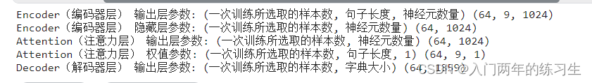
print ('Encoder（编码器层） 输出层参数: (一次训练所选取的样本数, 句子长度, 神经元数量) {}'.format(sample_output.shape))
print ('Encoder（编码器层） 隐藏层参数: (一次训练所选取的样本数, 神经元数量) {}'.format(sample_hidden.shape))  
attention_layer = BahdanauAttention(10)
attention_result, attention_weights = attention_layer(sample_hidden, sample_output)
print("Attention（注意力层） 输出层参数: (一次训练所选取的样本数, 神经元数量) {}".format(attention_result.shape))
print("Attention（注意力层） 权值参数: (一次训练所选取的样本数, 句子长度, 1) {}".format(attention_weights.shape))
decoder = Decoder(vocab_tar_size, embedding_dim, units, BATCH_SIZE)
sample_decoder_output, _, _ = decoder(tf.random.uniform((64, 1)),sample_hidden, sample_output)
print ('Decoder（解码器层） 输出层参数: (一次训练所选取的样本数, 字典大小) {}'.format(sample_decoder_output.shape))

在看一下我们模型设置的参数

大家可以进行微调，本人尝试过，效果影响不大。

三.模型训练

接下来有了模型，我们就可以进行训练了
简单来说训练注意力机制神经网络的步骤为：

1. 定义编码器-解码器模型架构，其中编码器用于将输入序列编码成一个固定长度的向量，解码器用于生成输出序列。
   2.定义一个注意力机制，用于在每个时间步根据编码器的输出和解码器的当前状态，计算一个上下文向量，该向量可以提供给解码器作为额外的信息用于生成输出序列。
   3在训练过程中，对于每个时间步，首先通过编码器获得输入序列的编码结果，然后将该编码结果和解码器的当前状态作为注意力机制的输入，得到上下文向量，将上下文向量和解码器的当前输入拼接在一起，通过解码器生成输出序列的概率分布。
   4.定义损失函数，通常使用交叉熵损失函数或者自定义损失函数，用于评估模型输出和真实输出之间的差距。
   5.使用反向传播算法计算梯度，并使用优化算法更新模型参数，使得损失函数最小化。
   6.在测试过程中，对于每个输入序列，使用训练好的模型预测输出序列，得到最终的结果。
   完整代码：

num_examples = 20000
path_to_file = '/kaggle/input/tansantcmn/cmn.txt'
BATCH_SIZE = 70
input_tensor, target_tensor, inp_lang, targ_lang = load_dataset(path_to_file, num_examples)
max_length_targ, max_length_inp = max_length(target_tensor),max_length(input_tensor)
input_tensor_train, input_tensor_val, target_tensor_train, target_tensor_val = train_test_split(input_tensor, target_tensor, test_size=0.2)
BUFFER_SIZE = len(input_tensor_train)
steps_per_epoch = len(input_tensor_train)//BATCH_SIZE
EPOCHS = 15
embedding_dim = 256
units = 1024
vocab_inp_size = len(inp_lang.word_index)+1
vocab_tar_size = len(targ_lang.word_index)+1
dataset = tf.data.Dataset.from_tensor_slices((input_tensor_train, target_tensor_train)).shuffle(BUFFER_SIZE)
dataset = dataset.batch(BATCH_SIZE, drop_remainder=True)  
encoder = Encoder(vocab_inp_size, embedding_dim, units, BATCH_SIZE)
attention_layer = BahdanauAttention(10)
decoder = Decoder(vocab_tar_size, embedding_dim, units, BATCH_SIZE)
optimizer = tf.keras.optimizers.Adam()
loss_object = tf.keras.losses.SparseCategoricalCrossentropy(from_logits=True, reduction='none')
#定义优化器和损失函数
def loss_function(real, pred):
    mask = tf.math.logical_not(tf.math.equal(real, 0))
    loss_ = loss_object(real, pred)
    mask = tf.cast(mask, dtype=loss_.dtype)
    loss_ *= mask
    return tf.reduce_mean(loss_)
#定义保存点
checkpoint_dir = './training_checkpoints'
checkpoint_prefix = os.path.join(checkpoint_dir, "ckpt")
checkpoint = tf.train.Checkpoint(optimizer=optimizer,
                                 encoder=encoder,
                                 decoder=decoder)
#TensorFlow 2.0引入的eager提高了代码的简洁性，但是性能略有损失。所以我们这里使用 @tf.function可以将eager模式转为高效的Graph模式，提高计算性能。
@tf.function
#定义一次训练中所要进行的工作:
def train_step(inp, targ, enc_hidden):
    #把损失初始化为0
    loss = 0
    with tf.GradientTape() as tape:
        # 把源语言（中文）输入编码器，并获得编码器的输出结果
        enc_output, enc_hidden = encoder(inp, enc_hidden)
        # 把编码器隐藏层数值，赋予解码器隐藏层，参与第一次的注意力计算
        dec_hidden = enc_hidden
        dec_input = tf.expand_dims([targ_lang.word_index['<start>']] * BATCH_SIZE, 1)
        #  循环目标句子中所有的词，将目标词作为下一个输入
        for t in range(1, targ.shape[1]):
            # 使用本单词、解码器的隐藏层、编码器的输出共同预测下一个单词。同时保留本次的解码器隐藏层，用于预测下一个词。
            predictions, dec_hidden, _ = decoder(dec_input, dec_hidden, enc_output)
            # 计算损失值，并累加。
            loss += loss_function(targ[:, t], predictions)
            # 使用teach_forcing
            # teach_forcing指的是，在训练时，每次解码器的输入并不是上次解码器的输出，而是样本目标语言对应单词。
            dec_input = tf.expand_dims(targ[:, t], 1)
        batch_loss = (loss / int(targ.shape[1]))
        # 需要训练参数是编码器的参数和解码的参数
        variables = encoder.trainable_variables + decoder.trainable_variables
        # 根据代价值计算下一次的参量值
        gradients = tape.gradient(loss, variables)
        # 将新的参量应用到模型
        optimizer.apply_gradients(zip(gradients, variables))
    return batch_loss

def evaluate(sentence):
     # 清空注意力图
    attention_plot = np.zeros((max_length_targ, max_length_inp))
    
     # 句子预处理
    sentence = preprocess_sentence(sentence)
    print(sentence)
    # 句子数字化
    inputs = [inp_lang.word_index[i] for i in sentence.split(' ')]
     # 按照最长句子长度补齐
    inputs = tf.keras.preprocessing.sequence.pad_sequences([inputs],maxlen=max_length_inp,padding='post')
    inputs = tf.convert_to_tensor(inputs)
    result = ''
    # 句子做编码
    hidden = [tf.zeros((1, units))]
    enc_out, enc_hidden = encoder(inputs, hidden)
     # 编码器隐藏层作为第一次解码器的隐藏层值
    dec_hidden = enc_hidden
    dec_input = tf.expand_dims([targ_lang.word_index['<start>']], 0)
    
    # 假设翻译结果不超过最长的样本句子
    for t in range(max_length_targ):
        
        # 逐个单词翻译
        predictions, dec_hidden, attention_weights = decoder(dec_input,dec_hidden,enc_out)
        # 存储注意力权重以便后面制图
        attention_weights = tf.reshape(attention_weights, (-1, ))
        attention_plot[t] = attention_weights.numpy()
        # 得到预测单词的字典编号
        predicted_id = tf.argmax(predictions[0]).numpy()
        # 从字典查到对应单词，用空格作分隔，与上一次结果进行拼接，组成翻译后的句子。
        result += targ_lang.index_word[predicted_id] + ' '
        # 如果是<end>表示翻译结束
        if targ_lang.index_word[predicted_id] == '<end>':
            return result, sentence, attention_plot
        # 预测的 ID 被保存起来，参与下一次预测。
        dec_input = tf.expand_dims([predicted_id], 0)
    return result, sentence, attention_plot
# 注意力权重制图函数
def plot_attention(attention, sentence, predicted_sentence):
    fig = plt.figure(figsize=(10,10))
    ax = fig.add_subplot(1, 1, 1)
    ax.matshow(attention, cmap='viridis')
    fontdict = {'fontsize': 14}
    ax.set_xticklabels([''] + sentence, fontdict=fontdict, rotation=90)
    ax.set_yticklabels([''] + predicted_sentence, fontdict=fontdict)
    ax.xaxis.set_major_locator(ticker.MultipleLocator(1))
    ax.yaxis.set_major_locator(ticker.MultipleLocator(1))
    plt.show()
#翻译一个句子。
def translate(sentence):
    result, sentence, attention_plot = evaluate(sentence)
    print('Input: %s' % (sentence))
    print('Predicted translation: {}'.format(result))
    attention_plot = attention_plot[:len(result.split(' ')), :len(sentence.split(' '))]
    plot_attention(attention_plot, sentence.split(' '), result.split(' '))

if __name__=="__main__":
    # checkpoint.restore(tf.train.latest_checkpoint(checkpoint_dir))
    for epoch in range(EPOCHS):
        start = time.time()
        # 初始化隐藏层和损失值
        enc_hidden = encoder.initialize_hidden_state()
        total_loss = 0
        # 一个批次的训练
        for (batch, (inp, targ)) in enumerate(dataset.take(steps_per_epoch)):
#            print("targ") 演示目标值张量，暂时注释掉
#            print(targ) 演示目标值张量，暂时注释掉
            batch_loss = train_step(inp, targ, enc_hidden)
            total_loss += batch_loss
            # 每100次显示一下模型损失值
            if batch % 100 == 0:
                print('Epoch {} Batch {} Loss {:.4f}'.format(epoch + 1,batch,batch_loss.numpy()))
        # 每 2 个周期（epoch），保存（检查点）一次模型
        if (epoch + 1) % 2 == 0:
            checkpoint.save(file_prefix = checkpoint_prefix)
        # 显示每次迭代的损失值和消耗时间
        print('Epoch {} Loss {:.4f}'.format(epoch + 1,total_loss / steps_per_epoch))
        print('Time taken for 1 epoch {} sec\n'.format(time.time() - start))
    #恢复检查点目录 （checkpoint_dir） 中最新的检查点
    checkpoint.restore(tf.train.latest_checkpoint(checkpoint_dir))
    translate('book')

这里要说的是训练的epoch尽量在50个以上，否则效果不是很明显。
比如这里我训练了15个epoch loss=0.0928

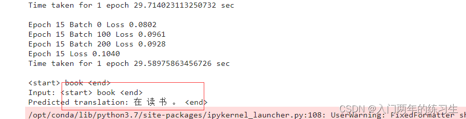
可以看到把（book）翻译为了（在读书）

这个是我训练了30个epoch loss=0.02

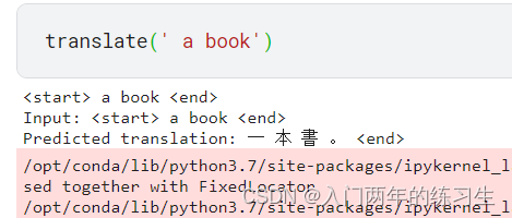
同样是翻译 a book 结果居然出了繁体字 哈哈哈！

---

总结

当训练epoch在60个左右时，可以发现训练的效果有显著的提高，但还是会存在有测试翻译错误的现象，这里可能是因为所给的数据集只有13444条，数据太少的缘故，所以大家可以去换一个数据集。在文章中给的代码是英译中，只需要将预处理函数 if not is_chinese(w):中的not去掉，就可以为中译英了。
如果文章中有错误，欢迎读者指出共同进步。