深度学习-LSTM预测未来值

**

用LSTM进行多输出预测

**
本文基于LSTM使用六小时（360分钟）的数据来预测10分钟后的发电量，主要就是讲解一下写代码过程中遇到的一些不太懂的地方，供同为萌新的参考，已经很了解深度学习的话，可以直接关闭了23333。本篇中使用的数据是经过数据筛选和处理的，有关数据筛选和处理的部分后续会上传。

1.参数列表

为了方便在不同情境下进行调参，易于其他人的使用，习惯性把一些需要修改的参数前置。首先选择读入文件的路径和文件名，再修改程序的工作路径到你文件所存储的位置（os.chdir(SaveFile_Path)），此处之所以要修改工作路径的原因是如果不加这条会默认程序执行在你程序所处的位置，后续存储文件时如果使用相对路径，会直接存储到python程序所在文件夹，如果对这个不介意这段可不加。*记得在输入存储位置时加上转义符r’’，否者会判定\为保留字。*然后再创建一个文件夹存储你所得到的那些结果，用if判断一下文件夹是否存在，如果不存在则创建一个。

接下来说一下时间步长的设置，使用LSTM网络，需要输入的数据格式为（样本数，时间步长，特征量），通俗的来理解就是，样本数指你有多少行数据，时间步长是指用多长的时间来预测，特征量指你样本中的特征量有多少个。time_step在工程实践上最多在250-500，超出范围会消耗过多计算量，delay指你要预测多少时间后的，数值越大，预测的准确性越低，batchsize，计算机一次处理多少数据之后计算损失函数，越大对计算机的性能要求越高，each_epoch循环计算多少次，lr后面keras.optimizers.Adam优化器中的学习率，初始学习率大概在0.01-0.001，过小会导致收敛速度慢，浪费计算资源，过大会导致损失函数震荡无法收敛。

'''修改数据'''
SaveFile_Path = r'D:\Desktop\2018年5MW运行数据\2018年\随机森林挑选特征'  # 要读取和保存的文件路径
readname = '201803-12随机森林特征量.csv'  #读取文件的名字
savename = r'201803-12特征量.csv'
os.chdir(SaveFile_Path)  # 修改当前工作目录

DIR = 'LSTM'
if not os.path.exists(DIR):  #判断括号里的文件是否存在的意思，括号内的可以是文件路径。
    os.makedirs(DIR)  #用于递归创建目录

TIME_STEP = 360 #时间步长360min 6h
DELAY = 10 #预测十分钟后
BATCHSZ = 5  #一个批处理(batch)大小
EACH_EPOCH = 3  #循环次数
LR = 0.001  #keras.optimizers.Adam中的学习率

2.绘制初始曲线

这部分没什么好说的，就是将你的数据绘制成图像，观察大致趋势。

'''
绘制初始数据曲线
'''
def plot_init():
    df = pd.read_csv(SaveFile_Path + '\\' + readname, header=0, index_col=0, encoding='gbk')
    values = df.values
    col = df.shape[1]
    plt.rcParams['font.sans-serif'] = ['SimHei']  # 用来正常显示中文标签
    plt.figure()
    for i in range(0, col):
        plt.subplot(col, 1, i+1)
        plt.plot(values[:, i])
        plt.title(df.columns[i], y=0.5, loc='right')
    plt.show()

3.LSTM数据准备

送入LSTM网络的数据格式必须是（样本数，时间步长，特征量），所以我们需要将数据处理一下。这里需要注意的是需要进行归一化，否则收敛困难。本文使用360min的数据去预测10min后的数据，总共21万行数据，20万用作训练，1万行作测试集，没有设置验证集。从数据中划分出标签，应为时间步长360min后的连续10min，接着时间步长窗口和标签窗口逐行滑动，生成LSTM的输入数据和标签。训练集使用随机种子进行伪随机打乱。函数返回train_X, train_y, test_X, test_y, scaler。

我在写的时候有疑惑的几个点：
fit_transform()的作用,与fit()、transform()的区别，这里简单介绍一下fit_transform()的作用，是对这部分数据先拟合，找到该part的整体指标，如均值、方差、最大值、最小值等等，然后对该trandata进行转换transform，从而实现数据的标准化、归一化，它是fit()、transform()的组合。之后可以用scaler.inverse_transform()将归一化的数据还原回去。

tf.random.set_seed(7)最开始我将import tensorflow as tf放在import部分的最下面报错说tensorflow中无random模块，之后将import tensorflow as tf往前移了几个错误消失，具体原因现在还没搞清楚，我觉得是前面导入模块对import tensorflow的影响。

'''
LSTM数据准备
'''

def train_test(timestep, nextstep):   #timestep时间步长, nextstep预测多长时间
    # load dataset
    dataset = pd.read_csv(SaveFile_Path + '\\' + readname, header=0, index_col=0, encoding='gbk')
    values = dataset.values
    # ensure all data is float
    values = values.astype('float32')
    # normalize features归一化
    scaler = MinMaxScaler(feature_range=(0, 1))  # sklearn 归一化函数
    scaled = scaler.fit_transform(values)  # fit_transform(X_train) 意思是找出X_train的均值和​​​​​​​标准差，并应用在X_train上。
    # split into train and test sets  将数据集进行划分，然后将训练集和测试集划分为输入和输出变量，最终将输入（X）改造为LSTM的输入格式，即[samples,timesteps,features]
    n_train_hours = 200000 #20万行作训练集，1万作测试集
    train = scaled[:n_train_hours, :]
    test = scaled[n_train_hours:, :]

    train_X = []
    train_y = []
    test_X = []
    test_y = []

    # 测试集：
    # 利用for循环，遍历整个测试集，提取测试集中连续360min的特征量作为输入特征test_X，第361-370min的发电量作为标签
    for i in range(len(train)-timestep-nextstep+1):
        train_X.append(train[i:(i+timestep), :])
        btemp = train[i+timestep:i+timestep+nextstep, 0]
        b = []
        for j in range(len(btemp)):
            b.append(btemp[j])
        train_y.append(b)

    # 对训练集进行打乱
    np.random.seed(7)
    np.random.shuffle(train_X)
    np.random.seed(7)
    np.random.shuffle(train_y)
    tf.random.set_seed(7)
    # 将训练集由list格式变为array格式
    train_X = np.array(train_X, dtype=np.float32)
    train_y = np.array(train_y, dtype=np.float32)

    # 使x_train符合RNN输入要求：[送入样本数， 循环核时间展开步数， 每个时间步输入特征个数]。
    # 此处整个数据集送入，送入样本数为train_X.shape[0]；输入360min数据，预测出第361min的发电量，循环核时间展开步数为360; 每个时间步送入的特征是某一min的运行数据，16个数据，故每个时间步输入特征个数为16
    train_X = np.reshape(train_X, (train_X.shape[0], 360, 16))

    # 测试集：
    # 利用for循环，遍历整个测试集，提取测试集中连续360min的特征量作为输入特征test_X，第361-370min的发电量作为标签
    for i in range(len(test)-timestep-nextstep+1):
        test_X.append(test[i:(i + timestep), :])
        btemp = test[i + timestep:i + timestep + nextstep, 0]
        b = []
        for j in range(len(btemp)):
            b.append(btemp[j])
        test_y.append(b)

    test_X, test_y = np.array(test_X, dtype=np.float32), np.array(test_y, dtype=np.float32)
    test_X = np.reshape(test_X, (test_X.shape[0], 360, 16))

    #print(train_X.shape, train_y.shape, test_X.shape, test_y.shape)
    return train_X, train_y, test_X, test_y, scaler

4.构造模型

模型构造这一块比较简单，主要是四个LSTM层再加一层全连接层，中间加了几个Dropout防止过拟合，神经元个数可以根据自己的需求进行调整，神经元个数越多，计算量越大。

def model_build(train_datas): #train_datas = train_X
    # LSTM层
    model = keras.models.Sequential()
    model.add(keras.layers.LSTM(40, input_shape=(train_datas.shape[1:]), return_sequences=True, )) #, return_sequences=True 400记忆体个数
    model.add(keras.layers.Dropout(0.1))
    model.add(keras.layers.LSTM(30, return_sequences=True)) # model.add(keras.layers.Dropout(0.5))
    model.add(keras.layers.Dropout(0.1))
    model.add(keras.layers.LSTM(40, return_sequences=True))
    model.add(keras.layers.Dropout(0.1))
    model.add(keras.layers.LSTM(40))
    model.add(keras.layers.BatchNormalization())  #批标准化：对一小批数据（batch）做标准化处理（使数据符合均值为0，标准差为1分布）
    model.add(keras.layers.Dense(train_y.shape[1]))   #全连接层
#配置训练方法
    model.compile(optimizer=keras.optimizers.Adam(lr=LR, amsgrad=True), loss='mse', metrics=[rmse])  # mae: mean_absolute_error

    return model

5.模型拟合

这里主要讲一下添加的一些函数，
model.load_weights(checkpoint_save_path) 先判断是否有训练过的模型，如果有加载模型继续进行训练。
keras.callbacks.ReduceLROnPlateau patience=4，连续4个batch_size损失函数没有变化就会调整学习率，新的学习率=旧的学习率*factor，min_lr当学习率小于这个数值时，循环停止。
keras.callbacks.ModelCheckpoint存储模型。
keras.callbacks.EarlyStopping连续15个batch_size损失函数没有变化，循环停止。

'''模型拟合'''
def model_fit(model, train_datas, train_labels,x_test, y_test):    #train_X, train_y, test_X, test_y


    checkpoint_save_path = "./checkpoint/LSTM_stock.ckpt" #模型保存位置

    if os.path.exists(checkpoint_save_path + '.index'):
        print('-------------load the model-----------------')
        model.load_weights(checkpoint_save_path)

    lr_reduce = keras.callbacks.ReduceLROnPlateau('val_loss',     #学习停止，模型会将学习率降低2-10倍，该hui
                                                  patience=4,
                                                  factor=0.7,
                                                  min_lr=0.00001)
    best_model = keras.callbacks.ModelCheckpoint(filepath=checkpoint_save_path,#保存模型
                                                 monitor='val_loss',
                                                 verbose=0,
                                                 save_best_only=True,
                                                 save_weights_only=True,
                                                 mode='min',
                                                 )

    early_stop = keras.callbacks.EarlyStopping(monitor='val_rmse', patience=15)

    history = model.fit(
        train_datas, train_labels,
        validation_data=(x_test, y_test),
        batch_size=BATCHSZ,
        epochs=EACH_EPOCH,
        verbose=2,
        callbacks=[
        best_model,
        early_stop,
        lr_reduce,
                    ]
    )

    loss = history.history['loss']
    val_loss = history.history['val_loss']
    #画出训练集和测试集的损失函数
    plt.plot(loss, label='Training Loss')
    plt.plot(val_loss, label='Validation Loss')
    plt.title('Training and Validation Loss')
    plt.legend()
    plt.savefig('./{}/{}.png'.format(DIR, '损失函数'))
    plt.close()

    return model, history

问题：编写代码时无法使用keras模型中的model.save(‘my_model.hdf5’)一直报错a bytes-like object is required, not ‘str’。这个问题我现在还没搞清是因为什么，所以我这里选择不使用它。

6.评价部分

评价部分主要使用两个指标，RMSE和R2_score。数据在之前已经进行过归一化，所以如果想还原真实的大小，需要使用scaler.inverse_transform()。关于这个函数有个小tip就是，需要把数据还原成原来使用fit_transform()时的shape，比如这里是二维的数据使用fit_transform()，那我使用scaler.inverse_transform()的数据列数shape[1]必须与前面的数据一致，shape[0]可以不一致。举个简单的例子：

import numpy as np
from sklearn.preprocessing import MinMaxScaler

data = np.array([
    [1, 8],
    [2, 7],
    [3, 6],
    [4, 7],
    ])
scaler = MinMaxScaler(feature_range=(0, 1))  # sklearn 归一化函数
scaled = scaler.fit_transform(data)
d2 = np.array([
    [0.2, 0.3],
    [0.1, 0.4]
])
d3 = scaler.inverse_transform(d2)
print(scaled)
print(d3)

d2和data的shape[1]一致，可以使用scaler.inverse_transform（）

[[0.         1.        ]
 [0.33333333 0.5       ]
 [0.66666667 0.        ]
 [1.         0.5       ]]
[[1.6 6.6]
 [1.3 6.8]]

这里我为了方便画图和进行数据分析，只取了预测的十个数据中的最后一个，也就是说我只关注预测的第10min的数据。

'''评价部分'''
def rmse(y_true, y_pred):  #sqrt求元素平方根  mean求张量平均值
    return keras.backend.sqrt(keras.backend.mean(keras.backend.square(y_pred - y_true), axis=-1))

def model_evaluation(model, test_X, test_y, savename):
    yhat = model.predict(test_X)
    yhat = yhat[:, -1]    #只取最后一个时刻的进行分析，1-9min的结果不是很重要
    y_normal = yhat.copy()
    y_normal[y_normal < 0] = 0  #将预测值归一化中小于0的都置0
    test_X = test_X[:, 0, :]
    test_y = test_y[:, -1]   #对应取test_y最后一个时刻

    #画出归一化后真实值和预测值的图像计算相关指标
    model_plot(test_y, y_normal, '归一化')
    RMSE_normal = np.sqrt(mean_squared_error(y_normal, test_y))
    R2_SCORE_normal = r2_score(y_normal, test_y)
    print('RMSE_normal: {}\nR2_SCORE_normal: {}\n'.format(RMSE_normal, R2_SCORE_normal))

    #返回计算归一化前
    yhat = yhat.reshape(len(yhat), 1)
    inv_yhat = concatenate((yhat, test_X[:, 1:]), axis=1)
    inv_y = scaler.inverse_transform(inv_yhat)  # 预测值转化
    y_pred = inv_y[:, 0]   #预测值由归一化值转为真实值
    y_pred[y_pred < 0] = 0  #将预测值真实值中小于0的都置0

    test_y = test_y.reshape((len(test_y), 1))
    inv_yact_hat = concatenate((test_y, test_X[:, 1:]), axis=1)
    inv_y = scaler.inverse_transform(inv_yact_hat)
    y_real = inv_y[:, 0]  # 标签由归一化值转为真实值
    '''
    在这里为什么进行比例反转，是因为我们将原始数据进行了预处理（连同输出值y），
    此时的误差损失计算是在处理之后的数据上进行的，为了计算在原始比例上的误差需要将数据进行转化。
    '''

    #存储真实值和预测值的相关信息
    y_pred_df = pd.DataFrame(index=y_pred)
    y_pred_df.to_csv(r'./{}/LSTM_pred.csv'.format(DIR), encoding='gbk', sep=',')
    y_real_df = pd.DataFrame(index=y_real)
    y_real_df.to_csv(r'./{}/LSTM_real.csv'.format(DIR), encoding='gbk', sep=',')

    # 画出真实值和预测值的图像并计算相关指标
    model_plot(y_real, y_pred, savename)
    RMSE = np.sqrt(mean_squared_error(y_pred, y_real))
    R2_SCORE = r2_score(y_pred, y_real)
    print('RMSE: {}\nR2_SCORE: {}\n'.format(RMSE, R2_SCORE))

    return RMSE, R2_SCORE, RMSE_normal, R2_SCORE_normal

7.保存模型信息和绘图

这部分没什么难点，比较简单，就是存储一下运行的结果。

'''保存模型信息'''
def model_save(RMSE, R2_SCORE, RMSE_normal, R2_SCORE_normal, savename):
    with open(r'./{}/LSTM.txt'.format(DIR), 'a') as fh:
        fh.write('参数设置：\nTIME_STEP: {}\tDELAY: {}\n'.format(TIME_STEP, DELAY))
        fh.write('RMSE: {}\nR2_SCORE: {}\n'.format(RMSE, R2_SCORE))
        fh.write('RMSE_normal: {}\nR2_SCORE: {}\n\n'.format(RMSE_normal, R2_SCORE_normal))
        print('%s模型信息保存成功！\n\n\n' % savename)

'''绘图相关'''
def model_plot(y_real, y_pred, savename):
    plt.cla()
    fig1 = plt.figure(figsize=(10, 14), dpi=80)
    plt.subplots_adjust(hspace=0.3)  #hspace=0.3为子图之间的空间保留的高度，平均轴高度的一部分.加了这个语句，子图会稍变小，因为空间也占用坐标轴的一部分

    ax1 = fig1.add_subplot(1, 1, 1)  # 1行x1列的网格里第一个
    ax1.plot(y_real, '-', c='blue', label='Real', linewidth=2)
    ax1.plot(y_pred, '-', c='red', label='Predict ', linewidth=2)
    ax1.legend(loc='upper right')
    ax1.set_xlabel('min')
    ax1.set_ylabel('KWH')
    ax1.grid()

    fig1.savefig('./{}/{}.png'.format(DIR, savename))
    plt.close()

8.结果部分

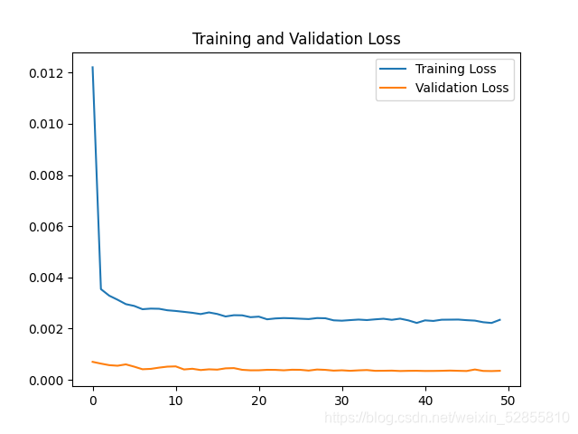
测试集损失函数比训练集好很多的原因可能是因为加入了Dropout，训练时开启，丢掉一部分数据集，测试时Dropout关闭。

使用了10万行数据训练，1万测试，RMSE=0.03。

9.全部代码

import tensorflow as tf
from tensorflow_core import keras
import os
import pandas as pd
import numpy as np
import matplotlib.pyplot as plt
from sklearn.preprocessing import MinMaxScaler
from sklearn.metrics import mean_squared_error, r2_score
from numpy import concatenate

pd.set_option('display.max_columns', None) #显示所有列

'''修改数据'''
SaveFile_Path = r''  # 此处加入读取和保存的文件路径
readname = ''  #读取文件的名字
savename = r''  #存储文件的名字
os.chdir(SaveFile_Path)  # 修改当前工作目录

DIR = 'LSTM'
if not os.path.exists(DIR):  #判断括号里的文件是否存在的意思，括号内的可以是文件路径。
    os.makedirs(DIR)  #用于递归创建目录

TIME_STEP = 360 #时间步长360min 6h
DELAY = 10 #预测十分钟后
BATCHSZ = 5  #一个批处理(batch)大小
EACH_EPOCH = 3  #循环次数
LR = 0.0001  #keras.optimizers.Adam中的学习率

'''
绘制初始数据曲线
'''
def plot_init():
    df = pd.read_csv(SaveFile_Path + '\\' + readname, header=0, index_col=0, encoding='gbk')
    values = df.values
    col = df.shape[1]
    plt.rcParams['font.sans-serif'] = ['SimHei']  # 用来正常显示中文标签
    plt.figure()
    for i in range(0, col):
        plt.subplot(col, 1, i+1)
        plt.plot(values[:, i])
        plt.title(df.columns[i], y=0.5, loc='right')
    plt.show()

'''
LSTM数据准备
'''

def train_test(timestep, nextstep):   #timestep时间步长, nextstep预测多长时间
    # load dataset
    dataset = pd.read_csv(SaveFile_Path + '\\' + readname, header=0, index_col=0, encoding='gbk')
    values = dataset.values
    # ensure all data is float
    values = values.astype('float32')
    # normalize features归一化
    scaler = MinMaxScaler(feature_range=(0, 1))  # sklearn 归一化函数
    scaled = scaler.fit_transform(values)  # fit_transform(X_train) 意思是找出X_train的均值和​​​​​​​标准差，并应用在X_train上。
    # split into train and test sets  将数据集进行划分，然后将训练集和测试集划分为输入和输出变量，最终将输入（X）改造为LSTM的输入格式，即[samples,timesteps,features]
    n_train_hours = 2000 #20万行作训练集，11万作测试集
    train = scaled[:n_train_hours, :]
    test = scaled[n_train_hours:3000, :]

    train_X = []
    train_y = []
    test_X = []
    test_y = []

    # 测试集：
    # 利用for循环，遍历整个测试集，提取测试集中连续360min的特征量作为输入特征test_X，第361-370min的发电量作为标签
    for i in range(len(train)-timestep-nextstep+1):
        train_X.append(train[i:(i+timestep), :])
        btemp = train[i+timestep:i+timestep+nextstep, 0]
        b = []
        for j in range(len(btemp)):
            b.append(btemp[j])
        train_y.append(b)

    # 对训练集进行打乱
    np.random.seed(7)
    np.random.shuffle(train_X)
    np.random.seed(7)
    np.random.shuffle(train_y)
    tf.random.set_seed(7)
    # 将训练集由list格式变为array格式
    train_X = np.array(train_X, dtype=np.float32)
    train_y = np.array(train_y, dtype=np.float32)

    # 使x_train符合RNN输入要求：[送入样本数， 循环核时间展开步数， 每个时间步输入特征个数]。
    # 此处整个数据集送入，送入样本数为train_X.shape[0]；输入360min数据，预测出第361min的发电量，循环核时间展开步数为360; 每个时间步送入的特征是某一min的运行数据，16个数据，故每个时间步输入特征个数为16
    train_X = np.reshape(train_X, (train_X.shape[0], 360, 16))

    # 测试集：
    # 利用for循环，遍历整个测试集，提取测试集中连续360min的特征量作为输入特征test_X，第361-370min的发电量作为标签
    for i in range(len(test)-timestep-nextstep+1):
        test_X.append(test[i:(i + timestep), :])
        btemp = test[i + timestep:i + timestep + nextstep, 0]
        b = []
        for j in range(len(btemp)):
            b.append(btemp[j])
        test_y.append(b)

    test_X, test_y = np.array(test_X, dtype=np.float32), np.array(test_y, dtype=np.float32)
    test_X = np.reshape(test_X, (test_X.shape[0], 360, 16))

    #print(train_X.shape, train_y.shape, test_X.shape, test_y.shape)
    return train_X, train_y, test_X, test_y, scaler

'''
构造模型
'''
def model_build(train_datas): #train_datas = train_X
    # LSTM层
    model = keras.models.Sequential()
    model.add(keras.layers.LSTM(40, input_shape=(train_datas.shape[1:]), return_sequences=True, )) #, return_sequences=True 400记忆体个数
    model.add(keras.layers.Dropout(0.1))
    model.add(keras.layers.LSTM(30, return_sequences=True)) # model.add(keras.layers.Dropout(0.5))
    model.add(keras.layers.Dropout(0.1))
    model.add(keras.layers.LSTM(40, return_sequences=True))
    model.add(keras.layers.Dropout(0.1))
    model.add(keras.layers.LSTM(40))
    model.add(keras.layers.BatchNormalization())  #批标准化：对一小批数据（batch）做标准化处理（使数据符合均值为0，标准差为1分布）
    model.add(keras.layers.Dense(train_y.shape[1]))   #全连接层
#配置训练方法
    model.compile(optimizer=keras.optimizers.Adam(lr=LR, amsgrad=True), loss='mse', metrics=[rmse])  # mae: mean_absolute_error

    return model

'''模型拟合'''
def model_fit(model, train_datas, train_labels,x_test, y_test):    #train_X, train_y, test_X, test_y


    checkpoint_save_path = "./checkpoint/LSTM_stock.ckpt" #模型保存位置

    if os.path.exists(checkpoint_save_path + '.index'):
        print('-------------load the model-----------------')
        model.load_weights(checkpoint_save_path)

    lr_reduce = keras.callbacks.ReduceLROnPlateau('val_loss',     #学习停止，模型会将学习率降低2-10倍，该hui
                                                  patience=4,
                                                  factor=0.7,
                                                  min_lr=0.00001)
    best_model = keras.callbacks.ModelCheckpoint(filepath=checkpoint_save_path,#保存模型
                                                 monitor='val_loss',
                                                 verbose=0,
                                                 save_best_only=True,
                                                 save_weights_only=True,
                                                 mode='min',
                                                 )

    early_stop = keras.callbacks.EarlyStopping(monitor='val_rmse', patience=15)

    history = model.fit(
        train_datas, train_labels,
        validation_data=(x_test, y_test),
        batch_size=BATCHSZ,
        epochs=EACH_EPOCH,
        verbose=2,
        callbacks=[
        best_model,
        early_stop,
        lr_reduce,
                    ]
    )

    loss = history.history['loss']
    val_loss = history.history['val_loss']
    #画出训练集和测试集的损失函数
    plt.plot(loss, label='Training Loss')
    plt.plot(val_loss, label='Validation Loss')
    plt.title('Training and Validation Loss')
    plt.legend()
    plt.savefig('./{}/{}.png'.format(DIR, '损失函数'))
    plt.close()

    return model, history

'''评价部分'''
def rmse(y_true, y_pred):  #sqrt求元素平方根  mean求张量平均值
    return keras.backend.sqrt(keras.backend.mean(keras.backend.square(y_pred - y_true), axis=-1))

def model_evaluation(model, test_X, test_y, savename):
    yhat = model.predict(test_X)
    yhat = yhat[:, -1]    #只取最后一个时刻的进行分析，1-9min的结果不是很重要
    y_normal = yhat.copy()
    y_normal[y_normal < 0] = 0  #将预测值归一化中小于0的都置0
    test_X = test_X[:, 0, :]
    test_y = test_y[:, -1]   #对应取test_y最后一个时刻

    #画出归一化后真实值和预测值的图像计算相关指标
    model_plot(test_y, y_normal, '归一化')
    RMSE_normal = np.sqrt(mean_squared_error(y_normal, test_y))
    R2_SCORE_normal = r2_score(y_normal, test_y)
    print('RMSE_normal: {}\nR2_SCORE_normal: {}\n'.format(RMSE_normal, R2_SCORE_normal))

    #返回计算归一化前
    yhat = yhat.reshape(len(yhat), 1)
    inv_yhat = concatenate((yhat, test_X[:, 1:]), axis=1)
    inv_y = scaler.inverse_transform(inv_yhat)  # 预测值转化
    y_pred = inv_y[:, 0]   #预测值由归一化值转为真实值
    y_pred[y_pred < 0] = 0  #将预测值真实值中小于0的都置0

    test_y = test_y.reshape((len(test_y), 1))
    inv_yact_hat = concatenate((test_y, test_X[:, 1:]), axis=1)
    inv_y = scaler.inverse_transform(inv_yact_hat)
    y_real = inv_y[:, 0]  # 标签由归一化值转为真实值
    '''
    在这里为什么进行比例反转，是因为我们将原始数据进行了预处理（连同输出值y），
    此时的误差损失计算是在处理之后的数据上进行的，为了计算在原始比例上的误差需要将数据进行转化。
    同时笔者有个小Tips：就是反转时的矩阵大小一定要和原来的大小（shape）完全相同，否则就会报错。
    '''

    #存储真实值和预测值的相关信息
    y_pred_df = pd.DataFrame(index=y_pred)
    y_pred_df.to_csv(r'./{}/LSTM_pred.csv'.format(DIR), encoding='gbk', sep=',')
    y_real_df = pd.DataFrame(index=y_real)
    y_real_df.to_csv(r'./{}/LSTM_real.csv'.format(DIR), encoding='gbk', sep=',')

    # 画出真实值和预测值的图像并计算相关指标
    model_plot(y_real, y_pred, savename)
    RMSE = np.sqrt(mean_squared_error(y_pred, y_real))
    R2_SCORE = r2_score(y_pred, y_real)
    print('RMSE: {}\nR2_SCORE: {}\n'.format(RMSE, R2_SCORE))

    return RMSE, R2_SCORE, RMSE_normal, R2_SCORE_normal

'''保存模型信息'''
def model_save(RMSE, R2_SCORE, RMSE_normal, R2_SCORE_normal, savename):
    with open(r'./{}/LSTM.txt'.format(DIR), 'a') as fh:
        fh.write('参数设置：\nTIME_STEP: {}\tDELAY: {}\n'.format(TIME_STEP, DELAY))
        fh.write('RMSE: {}\nR2_SCORE: {}\n'.format(RMSE, R2_SCORE))
        fh.write('RMSE_normal: {}\nR2_SCORE: {}\n\n'.format(RMSE_normal, R2_SCORE_normal))
        print('%s模型信息保存成功！\n\n\n' % savename)

'''绘图相关'''
def model_plot(y_real, y_pred, savename):
    plt.cla()
    fig1 = plt.figure(figsize=(10, 14), dpi=80)
    plt.subplots_adjust(hspace=0.3)  #hspace=0.3为子图之间的空间保留的高度，平均轴高度的一部分.加了这个语句，子图会稍变小，因为空间也占用坐标轴的一部分

    ax1 = fig1.add_subplot(1, 1, 1)  # 1行x1列的网格里第一个
    ax1.plot(y_real, '-', c='blue', label='Real', linewidth=2)
    ax1.plot(y_pred, '-', c='red', label='Predict ', linewidth=2)
    ax1.legend(loc='upper right')
    ax1.set_xlabel('min')
    ax1.set_ylabel('KWH')
    ax1.grid()

    fig1.savefig('./{}/{}.png'.format(DIR, savename))
    plt.close()

if __name__ == '__main__':
    #plot_init()  画初始数据图像
    train_X, train_y, test_X, test_y, scaler = train_test(timestep=360, nextstep=10)
    '''模型拟合'''
    model = model_build(train_X)
    model, history = model_fit(model, train_X, train_y, test_X, test_y)
    '''训练集评估'''
    RMSE_list, R2_SCORE_list, RMSE_normal_list, R2_SCORE_normal_list = model_evaluation(model, train_X, train_y, '训练')

    '''测试集评估'''
    RMSE_list, R2_SCORE_list, RMSE_normal_list, R2_SCORE_normal_list = model_evaluation(model, test_X, test_y, '验证')
    model_save(RMSE_list, R2_SCORE_list, RMSE_normal_list, R2_SCORE_normal_list, '验证')

10.总结

以上，来自刚入门的小菜鸡，如果有描述不当的地方，欢迎指正，问就是我错了。

其实写完之后再回看整个过程，发现代码本身其实并不难，但是对刚入门的新人来说，不会的东西太多了，调参都不知道该咋调，所以花了好多时间才写出来，希望这篇文章可以帮到同新入门的小白~

还有部分疑问：无法使用keras模型中的model.save(‘my_model.hdf5’)一直报错a bytes-like object is required, not ‘str’。

完整代码上传至了github：https://github.com/sw1122/LSTM.git

model.save无法保存.hdf5格式的问题已经解决，是tensorflow2.0配置文件的缺陷，tensorflow2.3,2.4版本已修复。缺少decode，解决方法如图：

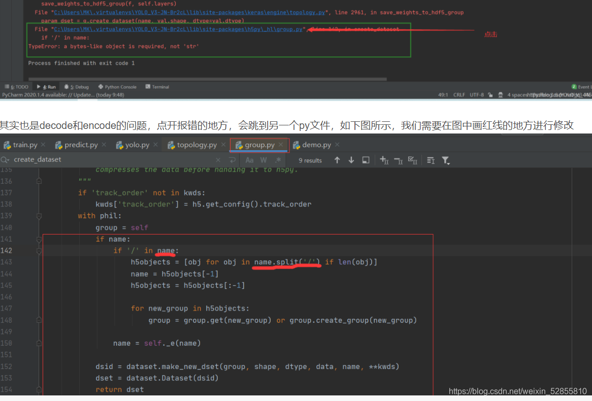
详情可以参考这篇博客：https://blog.csdn.net/qq_44644355/article/details/109411624