BERT源码解析-#notebook-code-CSDN博客

本文链接：https://blog.csdn.net/weixin_53162487/article/details/136736051

回顾:BERT结构

BERT模型结构基本上就是Transformer的Encoder部分，BERT-base对应的是12层encoder，BERT-large对应的是24层encoder.

BERT模型结构

在这里插入图片描述

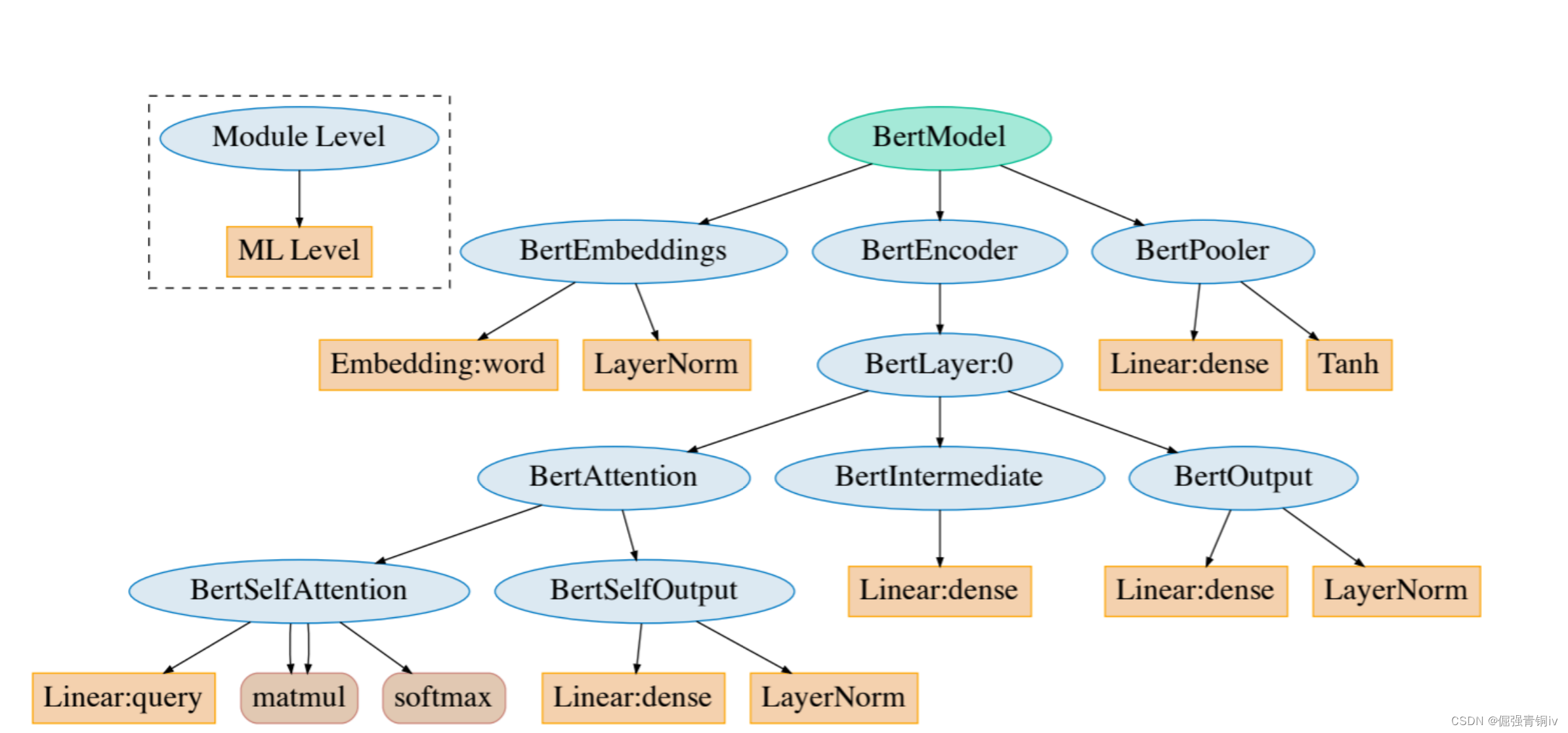
BERT Tokenization 分词模型（BertTokenizer）
BERT Model 本体模型（BertModel）

BertEmbeddings
BertEncoder
- BertLayer
  - BertAttention
  - BertIntermediate
  - BertOutput
BertPooler

BertTokenizer

Tokenizer是在自然语言处理（NLP）中的一个关键组件，它负责将文本转换成一种格式，以便机器学习模型能够理解和处理。
作用直白地说就是：
我们可以把Tokenizer比作是将一长串文字“切割”成有意义的小块（比如单词或字符）的工具。

Tokenizer的输入和输出

输入：Tokenizer的输入通常是原始文本。这可以是一句话、一个段落或者一个完整的文档。输入文本通常包含了自然语言的所有复杂性，如不同的语言、方言、专业术语、俚语等。
输出：Tokenizer的输出是一系列tokens，这些tokens已经被转换成了一种结构化的格式。输出的形式依赖于

Tokenizer的设计和目的，常见的有：

Token序列：一系列分割后的文本单元（如单词或字符）。
数字ID序列：如果Tokenizer包括编码过程，每个token会被映射到一个唯一的数字ID，这些ID对应于模型中的词汇表。
向量序列：在某些高级应用中，每个token可能直接被转换为一个稠密向量，这通常发生在使用预训练的嵌入模型时。

class BertTokenizer(PreTrainedTokenizer):
    """
    Construct a BERT tokenizer. Based on WordPiece.

    This tokenizer inherits from :class:`~transformers.PreTrainedTokenizer` which contains most of the main methods.
    Users should refer to this superclass for more information regarding those methods.
    ...
    """

BertTokenizer 是基于BasicTokenizer和WordPieceTokenizer的分词器：

BasicTokenizer负责处理的第一步——按标点、空格等分割句子，并处理是否统一小写，以及清理非法字符。
- 对于中文字符，通过预处理（加空格）来按字分割；
- 同时可以通过never_split指定对某些词不进行分割；
- 这一步是可选的（默认执行）。
WordPieceTokenizer在词的基础上，进一步将词分解为子词（subword）。
- subword 介于 char 和 word 之间，既在一定程度保留了词的含义，又能够照顾到英文中单复数、时态导致的词表爆炸和未登录词的 OOV（Out-Of-Vocabulary）问题，将词根与时态词缀等分割出来，从而减小词表，也降低了训练难度；
- 例如，tokenizer 这个词就可以拆解为“token”和“##izer”两部分，注意后面一个词的“##”表示接在前一个词后面。

BertTokenizer 有以下常用方法：

from_pretrained：从包含词表文件（vocab.txt）的目录中初始化一个分词器；
tokenize：将文本（词或者句子）分解为子词列表；
convert_tokens_to_ids：将子词列表转化为子词对应下标的列表；
convert_ids_to_tokens ：与上一个相反；
convert_tokens_to_string：将 subword 列表按“##”拼接回词或者句子；
encode：对于单个句子输入，分解词并加入特殊词形成“[CLS], x, [SEP]”的结构并转换为词表对应下标的列表；对于两个句子输入（多个句子只取前两个），分解词并加入特殊词形成“[CLS], x1, [SEP], x2, [SEP]”的结构并转换为下标列表；
decode：可以将 encode 方法的输出变为完整句子。
以及，类自身的方法：…

from transformers import BertTokenizer


tokenizer_dir = './pretrained_bert_models/bert_base_uncased/vocab.txt'
tokenizer = BertTokenizer(tokenizer_dir)
# 定义输入文本
text = "Hello, world! This is a test for the Tokenizer."
# 使用Tokenizer
encoded_input = tokenizer(text)
# 打印输出
print("原始文本:", text)
print("输出的内容:",encoded_input)
print("Tokenized 输出:", tokenizer.convert_ids_to_tokens(encoded_input['input_ids']))
print("数字ID序列:", encoded_input['input_ids'])
# 原始文本: Hello, world! This is a test for the Tokenizer.
# 输出的内容: {'input_ids': [101, 7592, 1010, 2088, 999, 2023, 2003, 1037, 3231, 2005, 1996, 19204, 17629, 1012, 102],
#             'token_type_ids': [0, 0, 0, 0, 0, 0, 0, 0, 0, 0, 0, 0, 0, 0, 0],
#             'attention_mask': [1, 1, 1, 1, 1, 1, 1, 1, 1, 1, 1, 1, 1, 1, 1]}
# Tokenized 输出: ['[CLS]', 'hello', ',', 'world', '!', 'this', 'is', 'a', 'test', 'for', 'the', 'token', '##izer', '.', '[SEP]']
# 数字ID序列: [101, 7592, 1010, 2088, 999, 2023, 2003, 1037, 3231, 2005, 1996, 19204, 17629, 1012, 102]

input_ids是模型理解文本的数字表示，列表中的每个整数代表词汇表中相应token的索引。例如，BERT模型中101和102分别标识句子开始和结束的特殊token。
token_type_ids用于区分输入序列的不同部分，如BERT中使用0和1来标记句子对中的第一个和第二个句子。
attention_mask是一个与input_ids长度相同的数组，其值为1的元素表示对应token是有效且应被模型关注的，而0则表示该token是填充或不重要的。这对于处理不同长度的输入序列至关重要。

BertModel

和 BERT 模型有关的代码主要写在/models/bert/modeling_bert.py中，这一份代码有一千多行，包含 BERT 模型的基本结构和基于它的微调模型等。

下面从 BERT 模型本体入手分析：

class BertModel(BertPreTrainedModel):
    """

    The model can behave as an encoder (with only self-attention) as well as a decoder, in which case a layer of
    cross-attention is added between the self-attention layers, following the architecture described in `Attention is
    all you need <https://arxiv.org/abs/1706.03762>`__ by Ashish Vaswani, Noam Shazeer, Niki Parmar, Jakob Uszkoreit,
    Llion Jones, Aidan N. Gomez, Lukasz Kaiser and Illia Polosukhin.

    To behave as an decoder the model needs to be initialized with the :obj:`is_decoder` argument of the configuration
    set to :obj:`True`. To be used in a Seq2Seq model, the model needs to initialized with both :obj:`is_decoder`
    argument and :obj:`add_cross_attention` set to :obj:`True`; an :obj:`encoder_hidden_states` is then expected as an
    input to the forward pass.
    """

BertModel 主要为 transformer encoder 结构，包含三个部分：

embeddings，即BertEmbeddings类的实体，根据单词符号获取对应的向量表示；
encoder，即BertEncoder类的实体；
pooler，即BertPooler类的实体，这一部分是可选的。

注意 BertModel 也可以配置为 Decoder，不过下文中不包含对这一部分的讨论。

下面将介绍 BertModel 的前向传播过程中各个参数的含义以及返回值：

def forward(
        self,
        input_ids=None,
        attention_mask=None,
        token_type_ids=None,
        position_ids=None,
        head_mask=None,
        inputs_embeds=None,
        encoder_hidden_states=None,
        encoder_attention_mask=None,
        past_key_values=None,
        use_cache=None,
        output_attentions=None,
        output_hidden_states=None,
        return_dict=None,
    ): ...

input_ids：经过 tokenizer 分词后的 subword 对应的下标列表；
attention_mask：在 self-attention 过程中，这一块 mask 用于标记 subword 所处句子和 padding 的区别，将 padding 部分填充为 0；
token_type_ids：标记 subword 当前所处句子（第一句/第二句/ padding）；
position_ids：标记当前词所在句子的位置下标；
head_mask：用于将某些层的某些注意力计算无效化；
inputs_embeds：如果提供了，那就不需要input_ids，跨过 embedding lookup 过程直接作为 Embedding 进入 Encoder 计算；
encoder_hidden_states：这一部分在 BertModel 配置为 decoder 时起作用，将执行 cross-attention 而不是 self-attention；
encoder_attention_mask：同上，在 cross-attention 中用于标记 encoder 端输入的 padding；
past_key_values：这个参数貌似是把预先计算好的 K-V 乘积传入，以降低 cross-attention 的开销（因为原本这部分是重复计算）；
use_cache：将保存上一个参数并传回，加速 decoding；
output_attentions：是否返回中间每层的 attention 输出；
output_hidden_states：是否返回中间每层的输出；
return_dict：是否按键值对的形式（ModelOutput 类，也可以当作 tuple 用）返回输出，默认为真。

注意，这里的 head_mask 对注意力计算的无效化，和下文提到的注意力头剪枝不同，而仅仅把某些注意力的计算结果给乘以这一系数。

输出部分如下：

# BertModel的前向传播返回部分
if not return_dict:
    return (sequence_output, pooled_output) + encoder_outputs[1:]

return BaseModelOutputWithPoolingAndCrossAttentions(
    last_hidden_state=sequence_output,
    pooler_output=pooled_output,
    past_key_values=encoder_outputs.past_key_values,
    hidden_states=encoder_outputs.hidden_states,
    attentions=encoder_outputs.attentions,
    cross_attentions=encoder_outputs.cross_attentions,
)

可以看出，返回值不但包含了 encoder 和 pooler 的输出，也包含了其他指定输出的部分（hidden_states 和 attention 等，这一部分在encoder_outputs[1:]）方便取用：

# BertEncoder的前向传播返回部分，即上面的encoder_outputs
if not return_dict:
    return tuple(
        v
        for v in [
            hidden_states,
            next_decoder_cache,
            all_hidden_states,
            all_self_attentions,
            all_cross_attentions,
        ]
        if v is not None
    )
return BaseModelOutputWithPastAndCrossAttentions(
    last_hidden_state=hidden_states,
    past_key_values=next_decoder_cache,
    hidden_states=all_hidden_states,
    attentions=all_self_attentions,
    cross_attentions=all_cross_attentions,
)

此外，BertModel 还有以下的方法，方便 BERT 玩家进行各种操作：

get_input_embeddings：提取 embedding 中的 word_embeddings 即词向量部分；
set_input_embeddings：为 embedding 中的 word_embeddings 赋值；
_prune_heads：提供了将注意力头剪枝的函数，输入为{layer_num: list of heads to prune in this layer}的字典，可以将指定层的某些注意力头剪枝。

剪枝是一个复杂的操作，需要将保留的注意力头部分的 Wq、Kq、Vq 和拼接后全连接部分的权重拷贝到一个新的较小的权重矩阵（注意先禁止 grad 再拷贝），并实时记录被剪掉的头以防下标出错。具体参考BertAttention部分的prune_heads方法.

BertEmbeddings

包含三个部分求和得到：
图：Bert-embedding

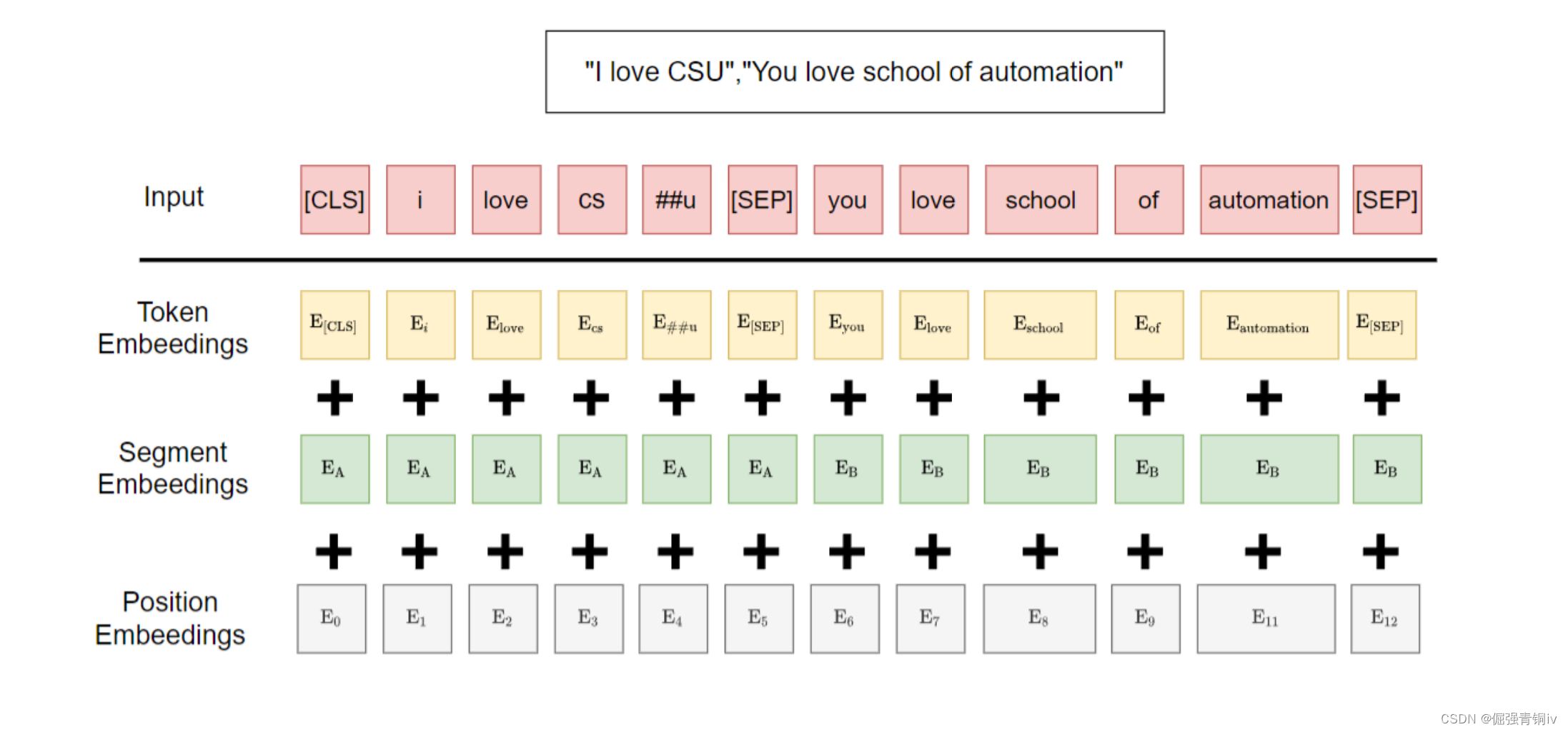
word_embeddings，上文中 subword 对应的嵌入。
token_type_embeddings，用于表示当前词所在的句子，辅助区别句子与 padding、句子对间的差异。
position_embeddings，句子中每个词的位置嵌入，用于区别词的顺序。和 transformer 论文中的设计不同，这一块是训练出来的，而不是通过 Sinusoidal 函数计算得到的固定嵌入。一般认为这种实现不利于拓展性（难以直接迁移到更长的句子中）。

三个 embedding 不带权重相加，并通过一层 LayerNorm+dropout 后输出，其大小为(batch_size, sequence_length, hidden_size)。

** 这里为什么要用 LayerNorm+Dropout 呢？为什么要用 LayerNorm 而不是 BatchNorm？可以参考一个不错的回答：transformer 为什么使用 layer normalization，而不是其他的归一化方法？**

要理解通过嵌入（embedding）层的输入和输出，我们可以使用一个预训练模型的嵌入层作为例子。这里，我们将继续使用Hugging Face的transformers库，并以BERT模型为例。嵌入层的主要作用是将输入的token ID转换成固定大小的向量，这些向量能够捕捉词汇的语义信息。

下面的代码将执行以下步骤：

从transformers库导入BERT模型和其Tokenizer。
初始化Tokenizer和模型。
定义一个文本输入，并用Tokenizer对其进行编码。
使用BERT模型的嵌入层对编码后的输入进行处理。
展示输入和输出。

from transformers import BertTokenizer, BertModel
import torch

# 初始化Tokenizer和模型
tokenizer = BertTokenizer.from_pretrained('bert-base-uncased')
model = BertModel.from_pretrained('bert-base-uncased')

# 定义文本输入
text = "Here is some text to encode"
encoded_input = tokenizer(text, return_tensors='pt')

# 提取编码后的输入IDs
input_ids = encoded_input['input_ids']

# 使用模型的嵌入层
with torch.no_grad():
    outputs = model.embeddings(input_ids)

# 展示输入和嵌入层的输出
print("Input IDs:", input_ids)
print("Output of Embedding Layer (shape):", outputs.shape)

在这个例子中：

输入（Input IDs）是文本经过Tokenizer处理后得到的input_ids，它是一个数字列表，每个数字代表文本中对应位置单词的唯一ID。
输出（Output of Embedding Layer）是嵌入层处理后的结果，它是一个多维张量，其形状为(batch_size, sequence_length, hidden_size)，其中：
- batch_size是输入批次的大小（如果你只输入了一句话，这个值就是1）。
- sequence_length是输入序列的长度。
- hidden_size是嵌入向量的维度，对于bert-base-uncased模型，这个值是768，意味着每个token都被转换成了一个768维的向量。

这个多维张量捕捉了输入文本的丰富语义信息，每个单词（token）都通过嵌入向量在一个高维空间中被表示，这些向量将作为模型下游任务的输入。

如果你想要进一步地观察token_embeddings，segment_embeddings，postion_embeddings,你可以这样做:

# 提取段ID和位置ID
token_type_ids = encoded_input['token_type_ids']
position_ids = torch.arange(input_ids.size(1)).unsqueeze(0)

# 使用模型的嵌入层
token_embeddings = model.embeddings.word_embeddings(input_ids)
segment_embeddings = model.embeddings.token_type_embeddings(token_type_ids)
position_embeddings = model.embeddings.position_embeddings(position_ids)

# 打印嵌入的形状
print("Token Embeddings shape:", token_embeddings.shape)
print("Segment Embeddings shape:", segment_embeddings.shape)
print("Position Embeddings shape:", position_embeddings.shape)

这里：

Token Embeddings (word_embeddings)：基于词汇表中每个token的ID，将每个token转换为一个固定大小的向量。
Segment Embeddings (token_type_embeddings)：用于区分两个不同的句子或文本片段。在简单的单句子输入中，这个嵌入向量可能不会提供很多信息，但在处理成对的句子（如问答任务）时很有用。
Position Embeddings (position_embeddings)：由于BERT使用的是Transformer架构，这个嵌入向量提供了每个token在句子中的位置信息，帮助模型理解单词顺序。

每种嵌入的形状都是(batch_size, sequence_length, hidden_size)，其中hidden_size对于bert-base-uncased模型是768，表示每个嵌入向量的维度。

BertEncoder

包含多层 BertLayer，这一块本身没有特别需要说明的地方，不过有一个细节值得参考：利用 gradient checkpointing 技术以降低训练时的显存占用。

gradient checkpointing 即梯度检查点，通过减少保存的计算图节点压缩模型占用空间，但是在计算梯度的时候需要重新计算没有存储的值，参考论文《Training Deep Nets with Sublinear Memory Cost》，过程如下示意图

请添加图片描述

图：gradient-checkpointing

在 BertEncoder 中，gradient checkpoint 是通过 torch.utils.checkpoint.checkpoint 实现的，使用起来比较方便，可以参考文档：torch.utils.checkpoint - PyTorch 1.8.1 documentation，这一机制的具体实现比较复杂，在此不作展开。

再往深一层走，就进入了 Encoder 的某一层：

BertLayer

BertAttention

本以为 attention 的实现就在这里，没想到还要再下一层……其中，self 成员就是多头注意力的实现，而 output 成员实现 attention 后的全连接 +dropout+residual+LayerNorm 一系列操作。

class BertAttention(nn.Module):
    def __init__(self, config):
        super().__init__()
        self.self = BertSelfAttention(config)
        self.output = BertSelfOutput(config)
        self.pruned_heads = set()

首先还是回到这一层。这里出现了上文提到的剪枝操作，即 prune_heads 方法：

 def prune_heads(self, heads):
        if len(heads) == 0:
            return
        heads, index = find_pruneable_heads_and_indices(
            heads, self.self.num_attention_heads, self.self.attention_head_size, self.pruned_heads
        )

        # Prune linear layers
        self.self.query = prune_linear_layer(self.self.query, index)
        self.self.key = prune_linear_layer(self.self.key, index)
        self.self.value = prune_linear_layer(self.self.value, index)
        self.output.dense = prune_linear_layer(self.output.dense, index, dim=1)

        # Update hyper params and store pruned heads
        self.self.num_attention_heads = self.self.num_attention_heads - len(heads)
        self.self.all_head_size = self.self.attention_head_size * self.self.num_attention_heads
        self.pruned_heads = self.pruned_heads.union(heads)

这里的具体实现概括如下：

find_pruneable_heads_and_indices是定位需要剪掉的 head，以及需要保留的维度下标 index；
prune_linear_layer则负责将 Wk/Wq/Wv 权重矩阵（连同 bias）中按照 index 保留没有被剪枝的维度后转移到新的矩阵。
接下来就到重头戏——Self-Attention 的具体实现。

BertSelfAttention

预警：这一块可以说是模型的核心区域，也是唯一涉及到公式的地方，所以将贴出大量代码。

初始化部分：

class BertSelfAttention(nn.Module):
    def __init__(self, config):
        super().__init__()
        if config.hidden_size % config.num_attention_heads != 0 and not hasattr(config, "embedding_size"):
            raise ValueError(
                "The hidden size (%d) is not a multiple of the number of attention "
                "heads (%d)" % (config.hidden_size, config.num_attention_heads)
            )

        self.num_attention_heads = config.num_attention_heads
        self.attention_head_size = int(config.hidden_size / config.num_attention_heads)
        self.all_head_size = self.num_attention_heads * self.attention_head_size

        self.query = nn.Linear(config.hidden_size, self.all_head_size)
        self.key = nn.Linear(config.hidden_size, self.all_head_size)
        self.value = nn.Linear(config.hidden_size, self.all_head_size)

        self.dropout = nn.Dropout(config.attention_probs_dropout_prob)
        self.position_embedding_type = getattr(config, "position_embedding_type", "absolute")
        if self.position_embedding_type == "relative_key" or self.position_embedding_type == "relative_key_query":
            self.max_position_embeddings = config.max_position_embeddings
            self.distance_embedding = nn.Embedding(2 * config.max_position_embeddings - 1, self.attention_head_size)

        self.is_decoder = config.is_decoder

class BertSelfAttention(nn.Module): 定义了一个名为 BertSelfAttention 的类，这个类继承自 PyTorch 的 nn.Module。这表明 BertSelfAttention 是一个神经网络模块，可以集成到更大的神经网络架构中。
def __init__(self, config): 这是类的构造函数，用于初始化 BertSelfAttention 实例。它接收一个配置对象 config，这个对象包含了模型配置的各种参数。
super().__init__(): 调用父类 nn.Module 的构造函数，进行必要的初始化操作。
检查 hidden_size 和 num_attention_heads 的兼容性：这部分代码确保隐藏层的大小 (hidden_size) 是注意力头的数量 (num_attention_heads) 的倍数。这是因为在计算自注意力时，隐藏层的输出需要被平均分配到每个注意力头上。
self.num_attention_heads = config.num_attention_heads: 定义注意力头的数量。
self.attention_head_size = int(config.hidden_size / config.num_attention_heads): 计算每个注意力头的大小。
self.all_head_size = self.num_attention_heads * self.attention_head_size: 计算所有注意力头的总大小。
self.query, self.key, self.value: 分别定义了用于生成查询（query）、键（key）和值（value）向量的线性变换。这些向量是自注意力机制中的核心组成部分。
self.dropout = nn.Dropout(config.attention_probs_dropout_prob): 定义了一个 Dropout 层，用于在注意力概率上应用 dropout，以减少过拟合。
self.position_embedding_type = getattr(config, "position_embedding_type", "absolute"): 获取位置嵌入类型，它决定了如何对位置信息进行编码。默认为 “absolute”。
if self.position_embedding_type == "relative_key" or self.position_embedding_type == "relative_key_query": 这段条件语句检查是否使用相对位置编码，如果是，则进行相应的初始化。
self.max_position_embeddings = config.max_position_embeddings: 设置最大位置嵌入数，这是相对位置编码所需的。
self.distance_embedding = nn.Embedding(2 * config.max_position_embeddings - 1, self.attention_head_size): 初始化用于相对位置编码的嵌入层。
self.is_decoder = config.is_decoder: 指示这个模块是否被用作解码器的一部分。在 Transformer 模型中，解码器用于生成输出序列，而编码器处理输入序列。
注意，hidden_size 和 all_head_size 在一开始是一样的。至于为什么要看起来多此一举地设置这一个变量——显然是因为上面那个剪枝函数，剪掉几个 attention head 以后 all_head_size 自然就小了；
hidden_size 必须是 num_attention_heads 的整数倍，以 bert-base 为例，每个 attention 包含 12 个 head，hidden_size 是 768，所以每个 head 大小即 attention_head_size=768/12=64；

然后是重点，也就是前向传播过程。

首先回顾一下 multi-head self-attention 的基本公式：

$D_k$ 表示key的维度; $D_m$ 表示token维度,T表示序列长度.
多头自注意力（Multi-HeadSelf-Attention），在多个不同的投影空间中捕捉不同的交互信息．假设在 $h$ 个投影空间中分别应用自注意力模型，有
$\begin{aligned} \operatorname{MultiHead}(\mathbf{Q},\mathbf{K},\mathbf{V})&=\boldsymbol{W}_o[\operatorname{head}_1;\cdots;\operatorname{head}_h],\\ \operatorname{head}_i&=\operatorname{self-att}(\boldsymbol{Q}_i,\boldsymbol{K}_i,\boldsymbol{V}_i),\\ \forall i\in\{1,\cdots,h\},\quad \boldsymbol{Q}_i&=\boldsymbol{W}_q^i\boldsymbol{Q},\boldsymbol{K}=\boldsymbol{W}_k^i\boldsymbol{K},\boldsymbol{V}=\boldsymbol{W}_v^i\boldsymbol{V},\end{aligned}$
其中 $\boldsymbol{W}_o \in \mathbb{R}^{D_m \times h D_v}$ 为输出投影矩阵， $\boldsymbol{W}_q^i \in \mathbb{R}^{D_k \times D_m}$ , $\boldsymbol{W}_k^i \in \mathbb{R}^{D_k \times D_m}$ , $\boldsymbol{W}_q^i \in \mathbb{R}^{D_v \times D_m}$ , 为投影矩阵， $\in \{ 1,...,h\}$ ，最终 $\operatorname{MultiHead}(\mathbf{Q},\mathbf{K},\mathbf{V}) \in \mathbb{R}^{D_m \times T}$
一般来说, $D_k,D_v,D_m$ 满足如下关系式子:
$D_k=D_v = D_m /h$
而自注意力模型 $\operatorname{self-att}$ 可以看作在一个线性投影空间中建立 $\mathbf{H}$ (自注意力中 $\mathbf{Q},\mathbf{K},\mathbf{V}均为\mathbf{H}$ )中不同向量之间的交互关系．其计算公式为
$\begin{aligned}\operatorname{self-att}(\boldsymbol{Q},\boldsymbol{K},\boldsymbol{V})&=\boldsymbol{V}\operatorname{softmax}\big(\frac{\boldsymbol{K}^\intercal\boldsymbol{Q}}{\sqrt{D_k}}\big),\\\boldsymbol{Q}&=\boldsymbol{W}_q\mathbf{H},\boldsymbol{K}=\boldsymbol{W}_k\mathbf{H},\boldsymbol{V}=\boldsymbol{W}_\upsilon\mathbf{H},\end{aligned}$

其中 $D_k$ 是输入矩阵 $\boldsymbol{Q}$ 和 $\boldsymbol{K}$ 中列向量的维度， $\boldsymbol{W}_q \in \mathbb{R}^{D_k \times D_m}$ , $\boldsymbol{W}_k \in \mathbb{R}^{D_k \times D_m}$ , $\boldsymbol{W}_v \in \mathbb{R}^{D_v \times D_m}$ 为三个投影矩阵。每一个 $\operatorname{self-att}(\boldsymbol{Q},\boldsymbol{K},\boldsymbol{V}) \in \mathbb{R}^{D_v \times T}$

而这些注意力头，众所周知是并行计算的，所以上面的 query、key、value 三个权重是唯一的——这并不是所有 heads 共享了权重，而是“拼接”起来了。

原论文中多头的理由为 Multi-head attention allows the model to jointly attend to information from different representation subspaces at different positions. With a single attention head, averaging inhibits this. 而另一个比较靠谱的分析有：为什么 Transformer 需要进行 Multi-head Attention？

看看 forward 方法：

def transpose_for_scores(self, x):
        new_x_shape = x.size()[:-1] + (self.num_attention_heads, self.attention_head_size)
        x = x.view(*new_x_shape)
        return x.permute(0, 2, 1, 3)

    def forward(
        self,
        hidden_states,
        attention_mask=None,
        head_mask=None,
        encoder_hidden_states=None,
        encoder_attention_mask=None,
        past_key_value=None,
        output_attentions=False,
    ):
        mixed_query_layer = self.query(hidden_states)

        # 省略一部分cross-attention的计算
        key_layer = self.transpose_for_scores(self.key(hidden_states))
        value_layer = self.transpose_for_scores(self.value(hidden_states))
        query_layer = self.transpose_for_scores(mixed_query_layer)

        # Take the dot product between "query" and "key" to get the raw attention scores.
        attention_scores = torch.matmul(query_layer, key_layer.transpose(-1, -2))
        # ...

这里的 transpose_for_scores 用来把 hidden_size 拆成多个头输出的形状，并且将中间两维转置以进行矩阵相乘；

这里 key_layer/value_layer/query_layer 的形状为：(batch_size, num_attention_heads, sequence_length, attention_head_size)；
这里 attention_scores 的形状为：(batch_size, num_attention_heads, sequence_length, sequence_length)，符合多个头单独计算获得的 attention map 形状。

到这里实现了 K 与 Q 相乘，获得 raw attention scores 的部分，按公式接下来应该是按 $d_k$ 进行 scaling 并做 softmax 的操作。然而先出现在眼前的是一个奇怪的positional_embedding，以及一堆爱因斯坦求和：

 # ...
        ''' 
        逻辑,一般的position_embedding_type是absolute绝对位置编码，
        这种绝对位置编码方法不能很好地处理长距离依赖关系，因为位置信息是固定的，不能表达不同位置之间的相对关系。
        "relative_key"和"relative_key_query"是两种常见的相对位置编码方式。
        在"relative_key"方法中，位置嵌入被添加到查询和键向量中，通过计算查询和键向量之间的相对距离来建模位置关系。
        在"relative_key_query"方法中，位置嵌入被添加到查询和键向量中，通过分别计算查询和键向量之间的相对距离来建模位置关系。
        
        '''
        if self.position_embedding_type == "relative_key" or self.position_embedding_type == "relative_key_query":
            # hidden_states : (batch_size, sequence_length, hidden_size)
            seq_length = hidden_states.size()[1]
            # position_ids_l: (sequence_length, 1)
            # position_ids_r: (1,sequence_length)
            position_ids_l = torch.arange(seq_length, dtype=torch.long, device=hidden_states.device).view(-1, 1)
            position_ids_r = torch.arange(seq_length, dtype=torch.long, device=hidden_states.device).view(1, -1)
            # 形状为(sequence_length, 1)的张量  - 形状为(1,sequence_length)的张量
            # 进行广播操作,position_ids_l和position_ids_r均被张成为(sequence_length, sequence_length)的张量
            # 而且对于position_ids_l而言，每一列都与第一列相同，为从0到sequence_length的连续序列；
            # 对于position_ids_r而言，每一行都与第一行相同，为从0到sequence_length的连续序列。
            # distance: (sequence_length,sequnece_length)
            distance = position_ids_l - position_ids_r
            '''  
            0, 0, 0, 0, 0           0, 1, 2, 3, 4, 5      0,-1,-2,-3,-4,-5
            1, 1, 1, 1, 1           0, 1, 2, 3, 4, 5      1, 0,-1,-2,-3,-4
            2, 2, 2, 2, 2,    -     0, 1, 2, 3, 4, 5   =  2, 1, 0,-1,-2,-3
            3, 3, 3, 3, 3           0, 1, 2, 3, 4, 5      3, 2, 1, 0,-1,-2
            4, 4, 4, 4, 4           0, 1, 2, 3, 4, 5      4, 3, 2, 1, 0,-1
            5, 5, 5, 5, 5           0, 1, 2, 3, 4, 5      5, 4, 3, 2, 1, 0           
            '''
            # self.max_position_embeddings - 1 => int 一般是511
            # distance + self.max_position_embeddings - 1 =>广播操作:每个元素都加上511
            # 维度仍然是(sequence_length,sequnece_length)
            # 经过self.distance_embedding处理得到形状为(sequence_length,sequnece_length,self.attention_head_size)的张量
            positional_embedding = self.distance_embedding(distance + self.max_position_embeddings - 1)
            positional_embedding = positional_embedding.to(dtype=query_layer.dtype)  # fp16 compatibility

            if self.position_embedding_type == "relative_key":
                # query_layer:bhld => (batch_size, num_heads, sequence_length, attention_head_size)
                # positional_embedding :lrd => (sequence_length, relative_position_dimensions ,attention_head_size)
                # 其中relative_position_dimensions = sequence_length
                # bhlr:(batch_size, num_heads, sequence_length, relative_position_dimensions) => (batch_size, num_heads, sequence_length,  sequence_length) 
                '''
                等价于如下过程:
                A = torch.randn(b,h,l,d)
                B = torch.randn(l,r,d)
                C = torch.zeros(b,h,l,r)
                for i in range(b):
                    for j in range(h):
                        for k in range(l):
                            for t in range(r):
                                C[i, j, k, t] = A[i,j,k,:] @ B[k,t,:] # 向量乘法=>点积
                '''
                # 
                relative_position_scores = torch.einsum("bhld,lrd->bhlr", query_layer, positional_embedding)
                attention_scores = attention_scores + relative_position_scores
            elif self.position_embedding_type == "relative_key_query":
                relative_position_scores_query = torch.einsum("bhld,lrd->bhlr", query_layer, positional_embedding)
                relative_position_scores_key = torch.einsum("bhrd,lrd->bhlr", key_layer, positional_embedding)
                attention_scores = attention_scores + relative_position_scores_query + relative_position_scores_key
        # ...

关于爱因斯坦求和约定，参考以下文档：torch.einsum - PyTorch 1.8.1 documentation

对于不同的positional_embedding_type，有三种操作：

absolute：默认值，这部分就不用处理；
relative_key：对 key_layer 作处理，将其与这里的positional_embedding和 key 矩阵相乘作为 key 相关的位置编码；
relative_key_query：对 key 和 value 都进行相乘以作为位置编码。

回到正常 attention 的流程：

# ...
        attention_scores = attention_scores / math.sqrt(self.attention_head_size)
        if attention_mask is not None:
            # Apply the attention mask is (precomputed for all layers in BertModel forward() function)
            attention_scores = attention_scores + attention_mask  # 这里为什么是+而不是*？

        # Normalize the attention scores to probabilities.
        attention_probs = nn.Softmax(dim=-1)(attention_scores)

        # This is actually dropping out entire tokens to attend to, which might
        # seem a bit unusual, but is taken from the original Transformer paper.
        attention_probs = self.dropout(attention_probs)

        # Mask heads if we want to
        if head_mask is not None:
            attention_probs = attention_probs * head_mask

        context_layer = torch.matmul(attention_probs, value_layer)

        context_layer = context_layer.permute(0, 2, 1, 3).contiguous()
        new_context_layer_shape = context_layer.size()[:-2] + (self.all_head_size,)
        context_layer = context_layer.view(*new_context_layer_shape)

        outputs = (context_layer, attention_probs) if output_attentions else (context_layer,)

        # 省略decoder返回值部分……
        return outputs

重大疑问：这里的attention_scores = attention_scores + attention_mask是在做什么？难道不应该是乘 mask 吗？

因为这里的 attention_mask 已经【被动过手脚】，将原本为 1 的部分变为 0，而原本为 0 的部分（即 padding）变为一个较大的负数，这样相加就得到了一个较大的负值：
至于为什么要用【一个较大的负数】？因为这样一来经过 softmax 操作以后这一项就会变成接近 0 的小数。

(Pdb) attention_mask
tensor([[[[    -0.,     -0.,     -0.,  ..., -10000., -10000., -10000.]]],
        [[[    -0.,     -0.,     -0.,  ..., -10000., -10000., -10000.]]],
        [[[    -0.,     -0.,     -0.,  ..., -10000., -10000., -10000.]]],
        ...,
        [[[    -0.,     -0.,     -0.,  ..., -10000., -10000., -10000.]]],
        [[[    -0.,     -0.,     -0.,  ..., -10000., -10000., -10000.]]],
        [[[    -0.,     -0.,     -0.,  ..., -10000., -10000., -10000.]]]],
       device='cuda:0')

那么，这一步是在哪里执行的呢？
在modeling_bert.py中没有找到答案，但是在modeling_utils.py中找到了一个特别的类：class ModuleUtilsMixin，在它的get_extended_attention_mask方法中发现了端倪：

 def get_extended_attention_mask(self, attention_mask: Tensor, input_shape: Tuple[int], device: device) -> Tensor:
        """
        Makes broadcastable attention and causal masks so that future and masked tokens are ignored.

        Arguments:
            attention_mask (:obj:`torch.Tensor`):
                Mask with ones indicating tokens to attend to, zeros for tokens to ignore.
            input_shape (:obj:`Tuple[int]`):
                The shape of the input to the model.
            device: (:obj:`torch.device`):
                The device of the input to the model.

        Returns:
            :obj:`torch.Tensor` The extended attention mask, with a the same dtype as :obj:`attention_mask.dtype`.
        """
        # 省略一部分……

        # Since attention_mask is 1.0 for positions we want to attend and 0.0 for
        # masked positions, this operation will create a tensor which is 0.0 for
        # positions we want to attend and -10000.0 for masked positions.
        # Since we are adding it to the raw scores before the softmax, this is
        # effectively the same as removing these entirely.
        extended_attention_mask = extended_attention_mask.to(dtype=self.dtype)  # fp16 compatibility
        extended_attention_mask = (1.0 - extended_attention_mask) * -10000.0
        return extended_attention_mask

那么，这个函数是在什么时候被调用的呢？和BertModel有什么关系呢？
OK，这里涉及到 BertModel 的继承细节了：BertModel继承自BertPreTrainedModel，后者继承自PreTrainedModel，而PreTrainedModel继承自[nn.Module, ModuleUtilsMixin, GenerationMixin]三个基类。——好复杂的封装！

这也就是说，BertModel必然在中间的某个步骤对原始的attention_mask调用了get_extended_attention_mask，导致attention_mask从原始的[1, 0]变为[0, -1e4]的取值。

最终在 BertModel 的前向传播过程中找到了这一调用（第 944 行）：

# We can provide a self-attention mask of dimensions [batch_size, from_seq_length, to_seq_length]
# ourselves in which case we just need to make it broadcastable to all heads.
extended_attention_mask: torch.Tensor = self.get_extended_attention_mask(attention_mask, input_shape, device)

问题解决了：这一方法不但实现了改变 mask 的值，还将其广播（broadcast）为可以直接与 attention map 相加的形状。
不愧是你，HuggingFace。

除此之外，值得注意的细节有：

按照每个头的维度进行缩放，对于 bert-base 就是 64 的平方根即 8；
attention_probs 不但做了 softmax，还用了一次 dropout，这是担心 attention 矩阵太稠密吗…… 这里也提到很不寻常，但是原始 Transformer 论文就是这么做的；
head_mask 就是之前提到的对多头计算的 mask，如果不设置默认是全 1，在这里就不会起作用；
context_layer 即 attention 矩阵与 value 矩阵的乘积，原始的大小为：(batch_size, num_attention_heads, sequence_length, attention_head_size) ；
context_layer 进行转置和 view 操作以后，形状就恢复了(batch_size, sequence_length, hidden_size)。

BertSelfOutput

class BertSelfOutput(nn.Module):
    def __init__(self, config):
        super().__init__()
        self.dense = nn.Linear(config.hidden_size, config.hidden_size)
        self.LayerNorm = nn.LayerNorm(config.hidden_size, eps=config.layer_norm_eps)
        self.dropout = nn.Dropout(config.hidden_dropout_prob)

    def forward(self, hidden_states, input_tensor):
        hidden_states = self.dense(hidden_states)
        hidden_states = self.dropout(hidden_states)
        hidden_states = self.LayerNorm(hidden_states + input_tensor)
        return hidden_states

这里又出现了 LayerNorm 和 Dropout 的组合，只不过这里是先 Dropout，进行残差连接后再进行 LayerNorm。至于为什么要做残差连接，最直接的目的就是降低网络层数过深带来的训练难度，对原始输入更加敏感～

BertIntermediate

看完了 BertAttention，在 Attention 后面还有一个全连接+激活的操作：

class BertIntermediate(nn.Module):
    def __init__(self, config):
        super().__init__()
        self.dense = nn.Linear(config.hidden_size, config.intermediate_size)
        if isinstance(config.hidden_act, str):
            self.intermediate_act_fn = ACT2FN[config.hidden_act]
        else:
            self.intermediate_act_fn = config.hidden_act

    def forward(self, hidden_states):
        hidden_states = self.dense(hidden_states)
        hidden_states = self.intermediate_act_fn(hidden_states)
        return hidden_states

这段代码定义了 BERT 模型中的另一个重要组件，即中间层（Intermediate layer），它通常位于自注意力层（如前述的 BertSelfAttention）和输出层之间。这个中间层的作用是对自注意力层的输出进行进一步的变换和激活，以增加模型的表达能力。下面是代码的具体解释：

class BertIntermediate(nn.Module): 定义了一个名为 BertIntermediate 的类，该类继承自 PyTorch 的 nn.Module 类。这表明 BertIntermediate 是一个神经网络模块。
def __init__(self, config): 类的构造函数。它接收一个配置对象 config，这个对象包含了模型配置的各种参数。
super().__init__(): 调用父类 nn.Module 的构造函数，进行必要的初始化操作。
self.dense = nn.Linear(config.hidden_size, config.intermediate_size): 定义了一个线性变换层，它将自注意力层的输出（维度为 hidden_size）映射到一个更高或更低的维度空间（intermediate_size）。这种映射有助于提高模型处理不同类型信息的能力。在bert中这里的全连接做了一个扩展，以 bert-base 为例，扩展维度为 3072，是原始维度 768 的 4 倍之多；
判断 config.hidden_act 的类型并获取激活函数：
- 如果 config.hidden_act 是一个字符串，那么通过查找预定义的激活函数字典 ACT2FN 来获取相应的激活函数。这个字典 ACT2FN 通常在模型的实现文件中定义，包含了如 ReLU、GELU 等常见的激活函数。
- 这里的激活函数默认实现为 gelu（Gaussian Error Linerar Units(GELUS）当然，它是无法直接计算的，可以用一个包含tanh的表达式进行近似（略)。
- 如果 config.hidden_act 不是字符串，直接将其作为激活函数。
def forward(self, hidden_states): 定义了模块的前向传播函数。hidden_states 参数是从上一层（如自注意力层）传递过来的隐藏状态。
- hidden_states = self.dense(hidden_states): 首先通过上面定义的线性变换层对输入的隐藏状态进行变换。
- hidden_states = self.intermediate_act_fn(hidden_states): 然后通过激活函数对线性变换后的结果进行非线性激活。
return hidden_states: 返回激活后的隐藏状态。

这个中间层（Intermediate layer）的设计理念是在自注意力机制提取的特征之上增加一层非线性变换，以增强模型的表达能力，从而能够捕捉到更加复杂的模式和关系。这种设计在 Transformer 架构的许多变体中都非常常见。

BertOutput

在这里又是一个全连接 +dropout+LayerNorm，还有一个残差连接 residual connect：

class BertOutput(nn.Module):
    def __init__(self, config):
        super().__init__()
        self.dense = nn.Linear(config.intermediate_size, config.hidden_size)
        self.LayerNorm = nn.LayerNorm(config.hidden_size, eps=config.layer_norm_eps)
        self.dropout = nn.Dropout(config.hidden_dropout_prob)

    def forward(self, hidden_states, input_tensor):
        hidden_states = self.dense(hidden_states)
        hidden_states = self.dropout(hidden_states)
        hidden_states = self.LayerNorm(hidden_states + input_tensor)
        return hidden_states

这里的操作和 BertSelfOutput 不能说没有关系，只能说一模一样…… 非常容易混淆的两个组件。

BERT 模型中两种不同的输出层：BertSelfOutput 和 BertOutput。尽管它们在结构和功能上非常相似，但主要区别在于它们所处理的数据和在模型中的位置。让我们详细解释一下这两者之间的差异：

BertSelfOutput 类

这个类是自注意力层的输出部分，其目的是对自注意力层的原始输出进行进一步处理。
线性层 (self.dense) 的输入和输出维度都是 config.hidden_size，意味着它的作用是在相同的维度空间内对数据进行转换。
它通常位于自注意力计算之后，用于在将数据传递给下一个层级之前，进行一次变换和标准化。

BertOutput 类

这个类设计用来处理中间层（BertIntermediate）的输出，并将其转换回模型的隐藏维度大小，以便继续后续的处理。
线性层 (self.dense) 的输入维度是 config.intermediate_size，输出维度是 config.hidden_size。这意味着它将从中间层的较大（或较小）维度空间映射回原始的隐藏维度空间。
这个类通常位于中间层（如BertIntermediate）之后，用于将经过非线性变换的数据恢复到原始的隐藏状态维度，以便进行后续的处理步骤。

共同点

两个类都使用了层归一化 (self.LayerNorm) 和 Dropout (self.dropout) 来进一步处理数据，以促进模型的训练稳定性和泛化能力。
它们的前向传播 (forward) 方法都包括了一个残差连接和层归一化的步骤，即将输入的 hidden_states 经过线性变换和 Dropout 处理后，与另一个输入的 input_tensor 相加，然后进行层归一化。

区别总结

主要区别在于它们处理的数据的维度和在模型中的位置不同：BertSelfOutput 用于处理自注意力层的输出，而 BertOutput 用于处理中间层的输出并将其转换回隐藏维度大小。
BertSelfOutput 中的线性变换保持输入和输出的维度不变，而 BertOutput 中的线性变换则负责将维度从 intermediate_size 转换回 hidden_size。

以下内容还包含基于 BERT 的应用模型，以及 BERT 相关的优化器和用法，将在下一篇文章作详细介绍。

BertPooler

这一层只是简单地取出了句子的第一个token，即[CLS]对应的向量，然后过一个全连接层和一个激活函数后输出：（这一部分是可选的，因为pooling有很多不同的操作）

class BertPooler(nn.Module):
    def __init__(self, config):
        super().__init__()
        self.dense = nn.Linear(config.hidden_size, config.hidden_size)
        self.activation = nn.Tanh()

    def forward(self, hidden_states):
        # We "pool" the model by simply taking the hidden state corresponding
        # to the first token.
        first_token_tensor = hidden_states[:, 0]
        pooled_output = self.dense(first_token_tensor)
        pooled_output = self.activation(pooled_output)
        return pooled_output

小总结

本小节对Bert模型的实现进行分析了学习，希望读者能对Bert实现有一个更为细致的把握。

值得注意的是，在 HuggingFace 实现的 Bert 模型中，使用了多种节约显存的技术：

gradient checkpoint，不保留前向传播节点，只在用时计算；apply_chunking_to_forward，按多个小批量和低维度计算 FFN 部分
BertModel 包含复杂的封装和较多的组件。以 bert-base 为例，主要组件如下：
- 总计Dropout出现了1+(1+1+1)x12=37次；
- 总计LayerNorm出现了1+(1+1)x12=25次；
  BertModel 有极大的参数量。以 bert-base 为例，其参数量为 109M。

参考

附录标准的bert模型结构大致如下

Layer: embeddings
BertEmbeddings(
  (word_embeddings): Embedding(30522, 768, padding_idx=0)
  (position_embeddings): Embedding(512, 768)
  (token_type_embeddings): Embedding(2, 768)
  (LayerNorm): LayerNorm((768,), eps=1e-12, elementwise_affine=True)
  (dropout): Dropout(p=0.1, inplace=False)
)
Layer: encoder
BertEncoder(
  (layer): ModuleList(
    (0): BertLayer(
      (attention): BertAttention(
        (self): BertSelfAttention(
          (query): Linear(in_features=768, out_features=768, bias=True)
          (key): Linear(in_features=768, out_features=768, bias=True)
          (value): Linear(in_features=768, out_features=768, bias=True)
          (dropout): Dropout(p=0.1, inplace=False)
        )
        (output): BertSelfOutput(
          (dense): Linear(in_features=768, out_features=768, bias=True)
          (LayerNorm): LayerNorm((768,), eps=1e-12, elementwise_affine=True)
          (dropout): Dropout(p=0.1, inplace=False)
        )
      )
      (intermediate): BertIntermediate(
        (dense): Linear(in_features=768, out_features=3072, bias=True)
        (intermediate_act_fn): GELUActivation()
      )
      (output): BertOutput(
        (dense): Linear(in_features=3072, out_features=768, bias=True)
        (LayerNorm): LayerNorm((768,), eps=1e-12, elementwise_affine=True)
        (dropout): Dropout(p=0.1, inplace=False)
      )
    )
    (1): BertLayer(
      (attention): BertAttention(
        (self): BertSelfAttention(
          (query): Linear(in_features=768, out_features=768, bias=True)
          (key): Linear(in_features=768, out_features=768, bias=True)
          (value): Linear(in_features=768, out_features=768, bias=True)
          (dropout): Dropout(p=0.1, inplace=False)
        )
        (output): BertSelfOutput(
          (dense): Linear(in_features=768, out_features=768, bias=True)
          (LayerNorm): LayerNorm((768,), eps=1e-12, elementwise_affine=True)
          (dropout): Dropout(p=0.1, inplace=False)
        )
      )
      (intermediate): BertIntermediate(
        (dense): Linear(in_features=768, out_features=3072, bias=True)
        (intermediate_act_fn): GELUActivation()
      )
      (output): BertOutput(
        (dense): Linear(in_features=3072, out_features=768, bias=True)
        (LayerNorm): LayerNorm((768,), eps=1e-12, elementwise_affine=True)
        (dropout): Dropout(p=0.1, inplace=False)
      )
    )
    (2): BertLayer(
      (attention): BertAttention(
        (self): BertSelfAttention(
          (query): Linear(in_features=768, out_features=768, bias=True)
          (key): Linear(in_features=768, out_features=768, bias=True)
          (value): Linear(in_features=768, out_features=768, bias=True)
          (dropout): Dropout(p=0.1, inplace=False)
        )
        (output): BertSelfOutput(
          (dense): Linear(in_features=768, out_features=768, bias=True)
          (LayerNorm): LayerNorm((768,), eps=1e-12, elementwise_affine=True)
          (dropout): Dropout(p=0.1, inplace=False)
        )
      )
      (intermediate): BertIntermediate(
        (dense): Linear(in_features=768, out_features=3072, bias=True)
        (intermediate_act_fn): GELUActivation()
      )
      (output): BertOutput(
        (dense): Linear(in_features=3072, out_features=768, bias=True)
        (LayerNorm): LayerNorm((768,), eps=1e-12, elementwise_affine=True)
        (dropout): Dropout(p=0.1, inplace=False)
      )
    )
    (3): BertLayer(
      (attention): BertAttention(
        (self): BertSelfAttention(
          (query): Linear(in_features=768, out_features=768, bias=True)
          (key): Linear(in_features=768, out_features=768, bias=True)
          (value): Linear(in_features=768, out_features=768, bias=True)
          (dropout): Dropout(p=0.1, inplace=False)
        )
        (output): BertSelfOutput(
          (dense): Linear(in_features=768, out_features=768, bias=True)
          (LayerNorm): LayerNorm((768,), eps=1e-12, elementwise_affine=True)
          (dropout): Dropout(p=0.1, inplace=False)
        )
      )
      (intermediate): BertIntermediate(
        (dense): Linear(in_features=768, out_features=3072, bias=True)
        (intermediate_act_fn): GELUActivation()
      )
      (output): BertOutput(
        (dense): Linear(in_features=3072, out_features=768, bias=True)
        (LayerNorm): LayerNorm((768,), eps=1e-12, elementwise_affine=True)
        (dropout): Dropout(p=0.1, inplace=False)
      )
    )
    (4): BertLayer(
      (attention): BertAttention(
        (self): BertSelfAttention(
          (query): Linear(in_features=768, out_features=768, bias=True)
          (key): Linear(in_features=768, out_features=768, bias=True)
          (value): Linear(in_features=768, out_features=768, bias=True)
          (dropout): Dropout(p=0.1, inplace=False)
        )
        (output): BertSelfOutput(
          (dense): Linear(in_features=768, out_features=768, bias=True)
          (LayerNorm): LayerNorm((768,), eps=1e-12, elementwise_affine=True)
          (dropout): Dropout(p=0.1, inplace=False)
        )
      )
      (intermediate): BertIntermediate(
        (dense): Linear(in_features=768, out_features=3072, bias=True)
        (intermediate_act_fn): GELUActivation()
      )
      (output): BertOutput(
        (dense): Linear(in_features=3072, out_features=768, bias=True)
        (LayerNorm): LayerNorm((768,), eps=1e-12, elementwise_affine=True)
        (dropout): Dropout(p=0.1, inplace=False)
      )
    )
    (5): BertLayer(
      (attention): BertAttention(
        (self): BertSelfAttention(
          (query): Linear(in_features=768, out_features=768, bias=True)
          (key): Linear(in_features=768, out_features=768, bias=True)
          (value): Linear(in_features=768, out_features=768, bias=True)
          (dropout): Dropout(p=0.1, inplace=False)
        )
        (output): BertSelfOutput(
          (dense): Linear(in_features=768, out_features=768, bias=True)
          (LayerNorm): LayerNorm((768,), eps=1e-12, elementwise_affine=True)
          (dropout): Dropout(p=0.1, inplace=False)
        )
      )
      (intermediate): BertIntermediate(
        (dense): Linear(in_features=768, out_features=3072, bias=True)
        (intermediate_act_fn): GELUActivation()
      )
      (output): BertOutput(
        (dense): Linear(in_features=3072, out_features=768, bias=True)
        (LayerNorm): LayerNorm((768,), eps=1e-12, elementwise_affine=True)
        (dropout): Dropout(p=0.1, inplace=False)
      )
    )
    (6): BertLayer(
      (attention): BertAttention(
        (self): BertSelfAttention(
          (query): Linear(in_features=768, out_features=768, bias=True)
          (key): Linear(in_features=768, out_features=768, bias=True)
          (value): Linear(in_features=768, out_features=768, bias=True)
          (dropout): Dropout(p=0.1, inplace=False)
        )
        (output): BertSelfOutput(
          (dense): Linear(in_features=768, out_features=768, bias=True)
          (LayerNorm): LayerNorm((768,), eps=1e-12, elementwise_affine=True)
          (dropout): Dropout(p=0.1, inplace=False)
        )
      )
      (intermediate): BertIntermediate(
        (dense): Linear(in_features=768, out_features=3072, bias=True)
        (intermediate_act_fn): GELUActivation()
      )
      (output): BertOutput(
        (dense): Linear(in_features=3072, out_features=768, bias=True)
        (LayerNorm): LayerNorm((768,), eps=1e-12, elementwise_affine=True)
        (dropout): Dropout(p=0.1, inplace=False)
      )
    )
    (7): BertLayer(
      (attention): BertAttention(
        (self): BertSelfAttention(
          (query): Linear(in_features=768, out_features=768, bias=True)
          (key): Linear(in_features=768, out_features=768, bias=True)
          (value): Linear(in_features=768, out_features=768, bias=True)
          (dropout): Dropout(p=0.1, inplace=False)
        )
        (output): BertSelfOutput(
          (dense): Linear(in_features=768, out_features=768, bias=True)
          (LayerNorm): LayerNorm((768,), eps=1e-12, elementwise_affine=True)
          (dropout): Dropout(p=0.1, inplace=False)
        )
      )
      (intermediate): BertIntermediate(
        (dense): Linear(in_features=768, out_features=3072, bias=True)
        (intermediate_act_fn): GELUActivation()
      )
      (output): BertOutput(
        (dense): Linear(in_features=3072, out_features=768, bias=True)
        (LayerNorm): LayerNorm((768,), eps=1e-12, elementwise_affine=True)
        (dropout): Dropout(p=0.1, inplace=False)
      )
    )
    (8): BertLayer(
      (attention): BertAttention(
        (self): BertSelfAttention(
          (query): Linear(in_features=768, out_features=768, bias=True)
          (key): Linear(in_features=768, out_features=768, bias=True)
          (value): Linear(in_features=768, out_features=768, bias=True)
          (dropout): Dropout(p=0.1, inplace=False)
        )
        (output): BertSelfOutput(
          (dense): Linear(in_features=768, out_features=768, bias=True)
          (LayerNorm): LayerNorm((768,), eps=1e-12, elementwise_affine=True)
          (dropout): Dropout(p=0.1, inplace=False)
        )
      )
      (intermediate): BertIntermediate(
        (dense): Linear(in_features=768, out_features=3072, bias=True)
        (intermediate_act_fn): GELUActivation()
      )
      (output): BertOutput(
        (dense): Linear(in_features=3072, out_features=768, bias=True)
        (LayerNorm): LayerNorm((768,), eps=1e-12, elementwise_affine=True)
        (dropout): Dropout(p=0.1, inplace=False)
      )
    )
    (9): BertLayer(
      (attention): BertAttention(
        (self): BertSelfAttention(
          (query): Linear(in_features=768, out_features=768, bias=True)
          (key): Linear(in_features=768, out_features=768, bias=True)
          (value): Linear(in_features=768, out_features=768, bias=True)
          (dropout): Dropout(p=0.1, inplace=False)
        )
        (output): BertSelfOutput(
          (dense): Linear(in_features=768, out_features=768, bias=True)
          (LayerNorm): LayerNorm((768,), eps=1e-12, elementwise_affine=True)
          (dropout): Dropout(p=0.1, inplace=False)
        )
      )
      (intermediate): BertIntermediate(
        (dense): Linear(in_features=768, out_features=3072, bias=True)
        (intermediate_act_fn): GELUActivation()
      )
      (output): BertOutput(
        (dense): Linear(in_features=3072, out_features=768, bias=True)
        (LayerNorm): LayerNorm((768,), eps=1e-12, elementwise_affine=True)
        (dropout): Dropout(p=0.1, inplace=False)
      )
    )
    (10): BertLayer(
      (attention): BertAttention(
        (self): BertSelfAttention(
          (query): Linear(in_features=768, out_features=768, bias=True)
          (key): Linear(in_features=768, out_features=768, bias=True)
          (value): Linear(in_features=768, out_features=768, bias=True)
          (dropout): Dropout(p=0.1, inplace=False)
        )
        (output): BertSelfOutput(
          (dense): Linear(in_features=768, out_features=768, bias=True)
          (LayerNorm): LayerNorm((768,), eps=1e-12, elementwise_affine=True)
          (dropout): Dropout(p=0.1, inplace=False)
        )
      )
      (intermediate): BertIntermediate(
        (dense): Linear(in_features=768, out_features=3072, bias=True)
        (intermediate_act_fn): GELUActivation()
      )
      (output): BertOutput(
        (dense): Linear(in_features=3072, out_features=768, bias=True)
        (LayerNorm): LayerNorm((768,), eps=1e-12, elementwise_affine=True)
        (dropout): Dropout(p=0.1, inplace=False)
      )
    )
    (11): BertLayer(
      (attention): BertAttention(
        (self): BertSelfAttention(
          (query): Linear(in_features=768, out_features=768, bias=True)
          (key): Linear(in_features=768, out_features=768, bias=True)
          (value): Linear(in_features=768, out_features=768, bias=True)
          (dropout): Dropout(p=0.1, inplace=False)
        )
        (output): BertSelfOutput(
          (dense): Linear(in_features=768, out_features=768, bias=True)
          (LayerNorm): LayerNorm((768,), eps=1e-12, elementwise_affine=True)
          (dropout): Dropout(p=0.1, inplace=False)
        )
      )
      (intermediate): BertIntermediate(
        (dense): Linear(in_features=768, out_features=3072, bias=True)
        (intermediate_act_fn): GELUActivation()
      )
      (output): BertOutput(
        (dense): Linear(in_features=3072, out_features=768, bias=True)
        (LayerNorm): LayerNorm((768,), eps=1e-12, elementwise_affine=True)
        (dropout): Dropout(p=0.1, inplace=False)
      )
    )
  )
)
Layer: pooler
BertPooler(
  (dense): Linear(in_features=768, out_features=768, bias=True)
  (activation): Tanh()
)