


两步移动搜索法(2SFCA)是一种比较常用的计算可达性的方法,具体原理省略,读者可自行学习。学堂君用R语言写了一个函数ToSFCA()来实现它,在这里分享给读者。读者若使用请注明出处,即本推文链接 。
1 数据准备及函数代码
1.1 数据准备
计算可达性需要的数据主要是两个矢量文件:一个是需求点(demand point,dp),可以为面或点对象;另一个是供给点(supply point,sp),一般为点对象。
属性要求:dp中应含有刻画其需求规模的属性变量(如人口规模);sp中应含有刻画其供给规模的属性变量。
1.2 ToSFCA()函数
学堂君编写的ToSFCA()函数的全部代码如下:
(读者若使用请注明出处,即本推文链接)
ToSFCA <- function(dp, sp, fun = c("inverse", "normal", "step"),
                   pop, size, r = NULL, r0 = 0,
                   dist = NULL, dist.output = F, ...) {
  require(sf)
  require(dplyr)
  require(tidyr)
  require(purrr)

  ## check input files
  if (is(dp, "Spatial")) dp <- st_as_sf(dp)
  if (is(sp, "Spatial")) sp <- st_as_sf(sp)
  if (!is(dp, "sf") | !is(sp, "sf")) {
    stop("`dp`和`sp`必须为矢量文件")
  }

  ## creat `id` for input object
  m = dim(dp)[1]
  n = dim(sp)[1]
  dp$dpid = 1:m
  sp$spid = 1:n

  ## distance matrix
  if (is.null(dist)) {
    dist <- st_distance(dp, sp) %>%
      as.data.frame() %>%
      set_names(1:n) %>%
      mutate(dpid = 1:m) %>%
      gather(key = "spid", value = "dist", -dpid) %>%
      map_df(as.numeric) %>%
      mutate(dist = dist/1000)
  } else dist.output = F

  if (dist.output) {
    message("输出结果为距离矩阵,请把它赋给`dist`参数并重新运行函数")
    return(dist) & break
  }

  dist = filter(dist, dist >= r0)
  if (!is.null(r)) dist = filter(dist, dist <= r)

  ## distance decay function
  inverse <- function(d, b = 2, min = 0, max = Inf) {
    d = data.frame(d = d, min = min, max = max)
    d = apply(d, 1, median)
    return(d^(-b))
  }

  normal <- function(d, sd = 1, min = 0, max = Inf) {
    d = data.frame(d = d, min = min, max = max)
    d = apply(d, 1, median)
    dnorm(d, sd = sd)
  }

  step <- function(d, step = NULL) {
    if (is.null(step)) step = quantile(d)
    step = c(min(d,step), step, max(d,step))
    step = unique(step)
    w = cut(d, breaks = step, include.lowest = T)
    w = as.integer(w)
    max(w) - w + 1
  }

  fun = get(fun[1])

  ## first step
  dp.df = st_drop_geometry(dp)[, c("dpid", pop)] %>% rename(pop = 2)
  sp.df = st_drop_geometry(sp)[, c("spid", size)] %>% rename(size = 2)
  dist = left_join(dist, dp.df, by = "dpid")
  ### rs: ratio of supply
  rs = dist %>%
    mutate(ad = pop*fun(dist,...)) %>%
    group_by(spid) %>%
    summarise(td = sum(ad)) %>%
    left_join(sp.df, by = "spid") %>%
    mutate(rs = size/td)

  ## second step
  Access = dist %>%
    left_join(sp.df, by = "spid") %>%
    left_join(rs, by = "spid") %>%
    mutate(as = rs*fun(dist,...)) %>%
    group_by(dpid) %>%
    summarise(access = sum(as))

  ## return result
  return(Access)
}
(读者若使用请注明出处,即本推文链接)
1.3 函数参数说明
函数参数说明如下:
dp:需求点文件;空间矢量数据(sp或sf对象);sp:供给点文件;空间矢量数据(sp或sf对象);fun:距离衰减函数的名称;内置了三种函数形式,支持自定义函数,使用方法见下文;字符串形式;pop:dp中表示需求规模的变量名称;字符串形式;size:sp中表示供给规模的变量名称;字符串形式;r:距离衰减函数的最大搜索半径,单位为千米;数值形式,可省略;r0:距离衰减函数的最小搜索半径,单位为千米;数值形式,默认值为0;dist:距离矩阵;使用方法见下文;数据框结构,可省略;dist.output:若该参数为TRUE,则函数输出结果为距离矩阵,使用方法见下文;逻辑形式,默认值为FALSE;...:所使用的距离衰减函数中的参数,使用方法见下文。
1.4 示例
准备模拟数据:
library(sf)
nc <- st_read(system.file("shape/nc.shp", package="sf"))
nc$pop <- 100

bbox <- st_bbox(nc)
set.seed(0723)
sp <- data.frame(
  x = runif(20, min = bbox[1], max = bbox[3]),
  y = runif(20, min = bbox[2], max = bbox[4]),
  size = 5
) %>%
  st_as_sf(coords = c("x", "y")) %>%
  st_set_crs(st_crs(nc))

plot(st_geometry(nc))
plot(st_geometry(sp), col = "red", add = T)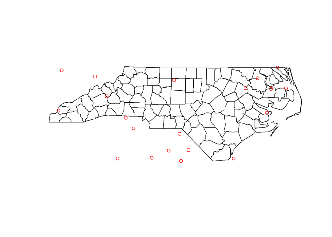
计算可达性并可视化:
Access <- ToSFCA(nc, sp, pop = "pop", size = "size", min = 1)
nc$access <- Access$access
plot(nc["access"])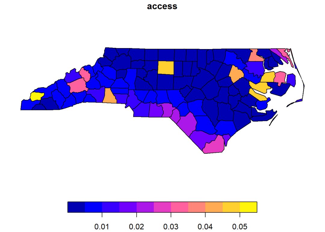
2 函数细节介绍
2.1 检查dp和sp
在R语言中,矢量数据有sp和sf两种形式,本函数是基于sf对象编写的;但用户也可以输入sp形式的对象,函数会将其转为sf对象。
若用户输入的dp或sp不是矢量数据(sp或sf形式),程序会停止运行并提醒用户“dp和sp必须为矢量文件”。
以下是这部分的代码:
require(sf)
## check input files
if (is(dp, "Spatial")) dp <- st_as_sf(dp)
if (is(sp, "Spatial")) sp <- st_as_sf(sp)
if (!is(dp, "sf") | !is(sp, "sf")) {
  stop("`dp`和`sp`必须为矢量文件")
}
2.2 距离矩阵
距离矩阵储存的是需求点和供给点之间的点对距离(若为面对象,使用其中心点代替)。
函数会根据dp和sp自动计算距离矩阵。但是计算距离矩阵相对比较费时,如果用户通过dist参数提供距离矩阵,则函数就不会再重复计算,而是直接使用输入的距离矩阵。
用户怎么准备距离矩阵呢?只要设置dist.output = TRUE,函数就会输出距离矩阵,用户再将其赋值给dist参数即可。用户一旦给dist参数赋值,dist.output参数就不再起作用。
如下代码所示,当dist.output = TRUE并且dist = NULL时,函数输出的将不是可达性,而是距离矩阵,并提醒用户“输出结果为距离矩阵,请把它赋给dist参数并重新运行函数”。
Dist <- ToSFCA(nc, sp, pop = "pop", size = "size", min = 1,
               dist.output = T)
Dist
## # A tibble: 2,000 × 3
##     dpid  spid  dist
##    <dbl> <dbl> <dbl>
##  1     1     1  259.
##  2     2     1  256.
##  3     3     1  232.
##  4     4     1  434.
##  5     5     1  328.
##  6     6     1  350.
##  7     7     1  417.
##  8     8     1  380.
##  9     9     1  284.
## 10    10     1  231.
## # … with 1,990 more rows
## # ℹ Use `print(n = ...)` to see more rows
以下是这部分的代码:
require(dplyr)
require(tidyr)
require(purrr)
## distance matrix
if (is.null(dist)) {
  dist <- st_distance(dp, sp) %>%
    as.data.frame() %>%
    set_names(1:n) %>%
    mutate(dpid = 1:m) %>%
    gather(key = "spid", value = "dist", -dpid) %>%
    map_df(as.numeric) %>%
    mutate(dist = dist/1000)
} else dist.output = F

if (dist.output) {
  message("输出结果为距离矩阵,请把它赋给`dist`参数并重新运行函数")
  return(dist) & break
}

dist = filter(dist, dist >= r0)
if (!is.null(r)) dist = filter(dist, dist <= r)
2.3 距离衰减函数
距离衰减函数表达了权重与距离呈反比的原理,本函数内置了三种衰减形式,分别为反距离函数("inverse")、正态函数("normal")、阶梯函数("step")。
2.3.1 反距离函数
反距离函数的表达式如下:
这部分的代码如下:
inverse <- function(d, b = 2, min = 0, max = Inf) {
  d = data.frame(d = d, min = min, max = max)
  d = apply(d, 1, median)
  return(d^(-b))
}
绘制其大致的函数图象:
x = seq(0,10,0.01)
w1 <- inverse(x, b = 0.5, min = 1, max = 5)
plot(x, w1, type = "l", family = "mono")
abline(v = 1, col = "grey", lty = 2)
abline(v = 5, col = "grey", lty = 2)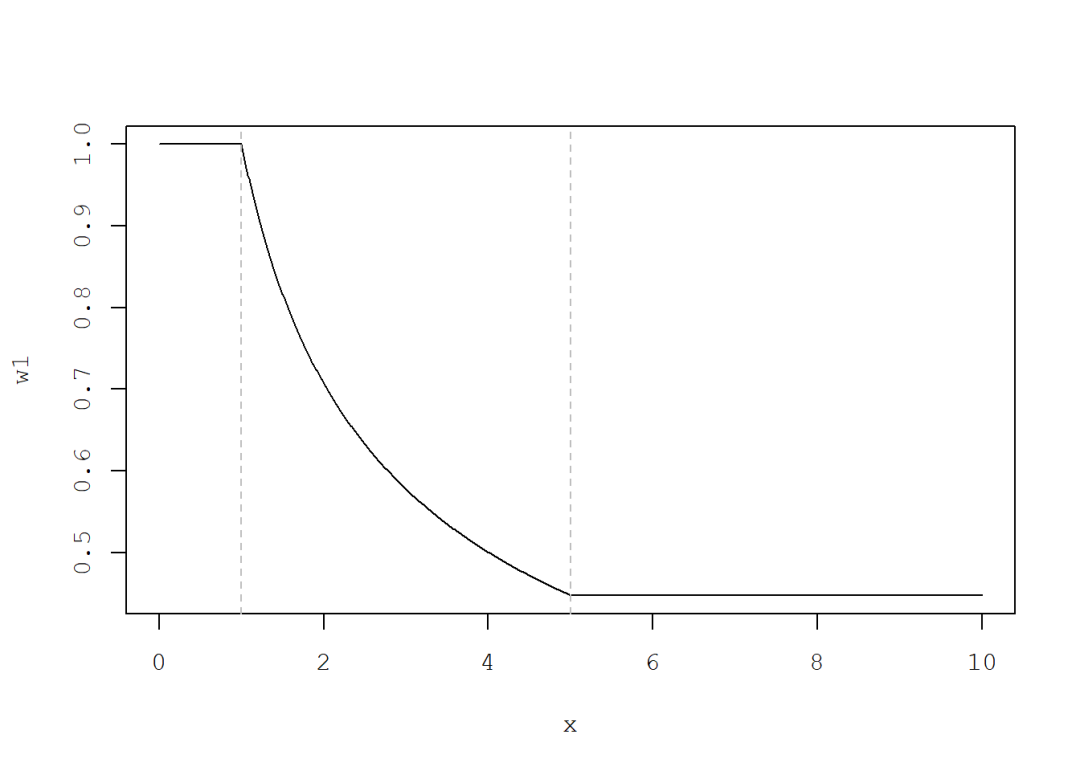
2.3.2 正态函数
正态分布的密度函数的右半部分。实现代码如下:
normal <- function(d, sd = 1, min = 0, max = Inf) {
  d = data.frame(d = d, min = min, max = max)
  d = apply(d, 1, median)
  dnorm(d, sd = sd)
}
sd:正态分布的标准差,默认为1。
绘制其大致的函数图象:
x = seq(0,10,0.01)
w2 <- normal(x, sd = 1.5, min = 1, max = 5)
plot(x, w2, type = "l", family = "mono")
abline(v = 1, col = "grey", lty = 2)
abline(v = 5, col = "grey", lty = 2)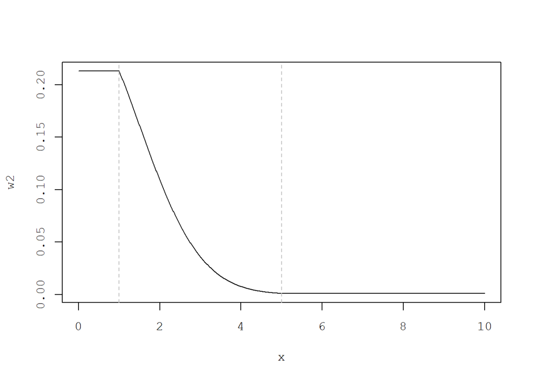
2.3.3 阶梯函数
实现代码如下,默认以距离的四分位点进行分段:
step <- function(d, step = NULL) {
  if (is.null(step)) step = quantile(d)
  step = c(min(d,step), step, max(d,step))
  step = unique(step)
  w = cut(d, breaks = step, include.lowest = T)
  w = as.integer(w)
  max(w) - w + 1
}
绘制其大致的函数图象:
x = seq(0,10,0.01)
w2 <- step(x, step = c(3,6,9))
plot(x, w2, type = "l", family = "mono")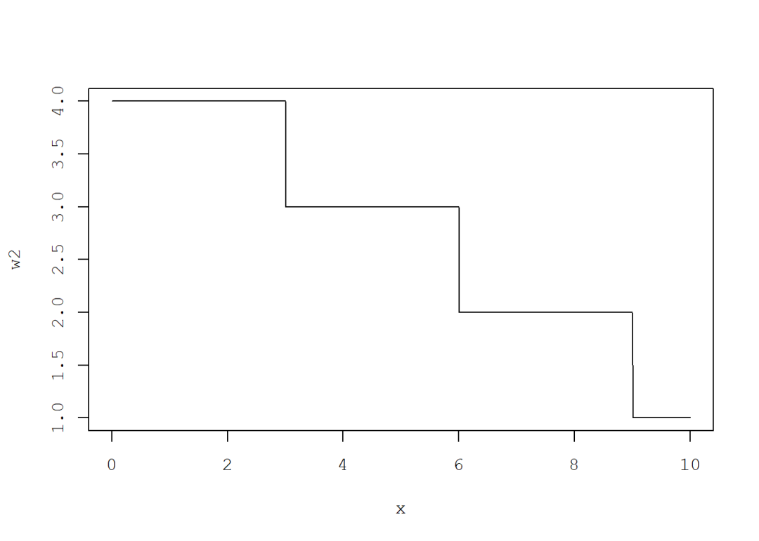
2.3.4 调用方法
本函数通过fun参数调用距离衰减函数,并会自动继承其所有参数(即...)。上述三个衰减函数为内置函数可以直接调用,默认值为"inverse"。衰减函数的参数除d以外都可以直接在本函数中使用。
比如,要调用阶梯函数,可以设置fun = "step",可以在本函数中使用它的step参数:
ToSFCA(nc, sp, pop = "pop", size = "size",
fun = "step", step = c(100, 500, 1000))需要注意的是,衰减函数中的参数需要对应。比如阶梯函数中没有min参数,如果用户在函数中设置了就会报错:
ToSFCA(nc, sp, pop = "pop", size = "size",
       fun = "step", step = c(100, 500, 1000),
       min = 1)
2.3.5 自定义函数
本函数接受用户自定义的距离衰减函数,其唯一要求是第一个参数必须为距离(不一定命名为d),其余参数可随意设置(但不能使用本函数的同名参数)。
用户自定义函数并在R中运行后即可调用,调用方法同内置函数,其参数也可在本函数中使用。
例如,定义一个名为fx的函数,使用x表示距离参数,para为衰减参数:
fx <- function(x, para) {
  x^(1/para)
}

## para为fx()中的参数
ToSFCA(nc, sp, pop = "pop", size = "size",
       fun = "fx", para = 2)
3 其他
读者在注明出处的前提下可自行使用。若发现计算结果有问题请及时联系学堂君。


 898
898

 被折叠的 条评论
为什么被折叠?
被折叠的 条评论
为什么被折叠?
 到【灌水乐园】发言


