


chapter1
function test1
format rat
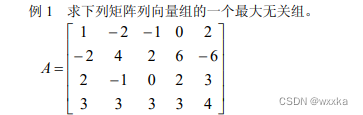
a=[1,-2,-1,0,2;
-2,4,2,6,-6;
2,-1,0,2,3;
3,3,3,3,4];
%求a的最大无关组
b=rref(a)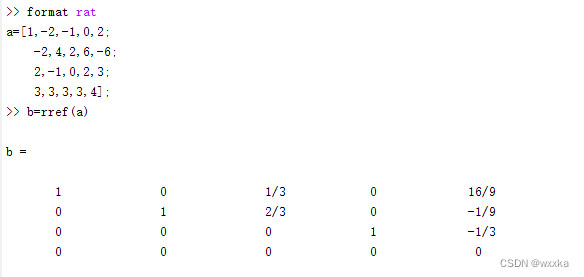
function test2
format rat
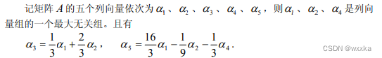
a=[2 2 -1;
2 -1 2;
-1 2 2];
%求a的最大无关组
b=[1 4;
0 3;
-4 2];
c=rref([a,b]);
%
% c =
%
% 1 0 0 2/3 4/3
% 0 1 0 -2/3 1
% 0 0 1 -1 2/3
%
b1=2/3*a(:,1)-2/3*a(:,2)-1*a(:,3)
b2=4/3*a(:,1)+1*a(:,2)+2/3*a(:,3)chapter2

![]()
![]()
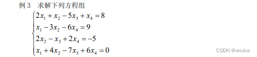
function test3

format rat
a=[2 1 -5 1;
   1 -3 0 -6;
   0 2 -1 2;
   1 4 -7 6];
%求a的最大无关组
b=[8;
    9;
    -5;
    0];

solution =a\b
%    3             -4             -1              1  %solution'
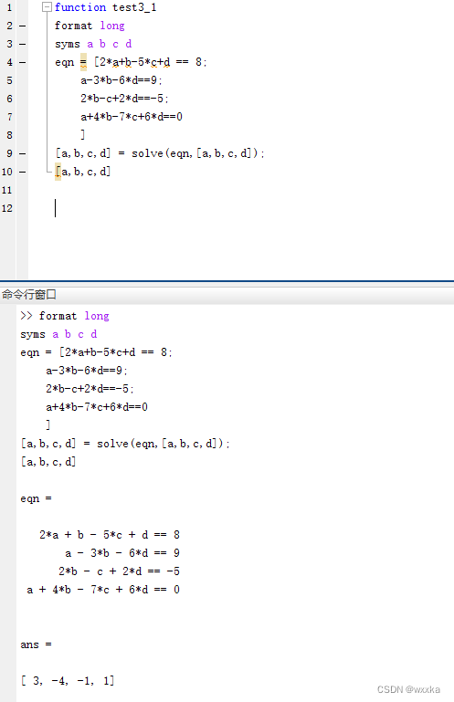
另一种解法---solve函数
function test3_1
format long
syms a b c d
eqn = [2*a+b-5*c+d == 8;
    a-3*b-6*d==9;
    2*b-c+2*d==-5;
    a+4*b-7*c+6*d==0
    ]
[a,b,c,d] = solve(eqn,[a,b,c,d]);
[a,b,c,d]
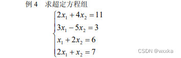
function test4
format rat
a=[2 4;
   3 -5;
   1 2;
   2 1];
%求a的最大无关组
b=[11;
    3;
    6;
    7];

solution =a\b
%    830/273        113/91   %solution'
a*solution
%
% ans =
%
%      232/21
%      265/91
%      116/21
%     1999/273
format long
a*solution
%
% ans =
%
%   11.047619047619046
%    2.912087912087914
%    5.523809523809523
%    7.322344322344321
从上面的结果,看出,并不能很好求出结果,对于求得结果,后两个等式基本不满足
function test4_1
format long
syms a b
eqn = [2*a + 4*b == 11;
    3*a-5*b==3;
    a+2*b==6;
    2*a+b==7];
[a,b] = solve(eqn,[a,b]);
[a,b]
只求解前三个等式
function test4_2
format rat
a=[2 4;
   3 -5;
   1 2;];
%求a的最大无关组
b=[11;
    3;
    6];

solution =a\b
%   3.090909090909089   1.254545454545454%solution'
a*solution
%
% ans =
%
%       56/5
%        3
%       28/5
format long
a*solution
%
% ans =
%
%   11.199999999999994
%    2.999999999999996
%    5.599999999999997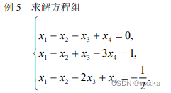
欠定方程
function test5_2

format rat
a=[1 -1 -1 1;
   1 -1 1 -3;
   1 -1 -2 1];
%求a的最大无关组
b=[0;
    1;
    -1/2];

solution =a\b
% solution =
%
%        0
%       -1/2
%        1/2
%        1/39831333786592880
利用最大线性无关组
function test5

format rat
a=[1 -1 -1 1;
   1 -1 1 -3;
   1 -1 -2 1];
%求a的最大无关组
b=[0;
    1;
    -1/2];
c=[a,b];
d=rref(c)
% solution =
%
%        0
%       -1/2
%        1/2
%        1/39831333786592880

% d =
%
%        1             -1              0              0              1/2
%        0              0              1              0              1/2
%        0              0              0              1              0

% a-b=0.5;
% c=0.5;
% d=0;
function test5_1
format long
syms a b c d
eqn = [a-b-c+d == 0;
a-b+c-3*d==1;
a-b-2*c+d==-0.5];
[a,b c d] = solve(eqn,[a,b c d]);
[a,b c d]
% ans =
%
% [ 1/2, 0, 1/2, 0]
function test6_1

x=str2sym('[a+sin(d),b;1/c,d]');
y=det(x)
%det(x)%返回x的行列式
%
% x=str2sym('[a+sin(d),b;1/c,d]');
% y=det(x)
%
% y =
%
% (a*c*d - b + c*d*sin(d))/c
function test6
syms a b c d
x=[a+sin(d),b;1/c,d];
y=det(x)
%det(x)%返回x的行列式
% y =
%
% (a*c*d - b + c*d*sin(d))/c

function test7
a=[2/3,sqrt(2);3,1];
b=sym(a)
%
% a=[2/3,sqrt(2);3,1];
% a
%
% a =
%
%        2/3         1393/985
%        3              1
%
% b=sym(a)
%
% b =
%
% [ 2/3, 2^(1/2)]
% [   3,       1]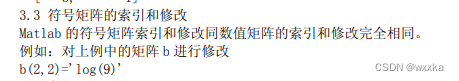
function test8
a=[2/3,sqrt(2);3,1];
b=sym(a)
%
% a=[2/3,sqrt(2);3,1];
% a
%
% a =
%
%        2/3         1393/985
%        3              1
%
% b=sym(a)
%
% b =
%
% [ 2/3, 2^(1/2)]
% [   3,       1]
b(2,2)=str2sym('log(9)')
%
% b(2,2)=str2sym('log(9)')
%
% b =
%
% [ 2/3, 2^(1/2)]
% [   3,  log(9)]
function test9
format rat
a=[0 1 1 -1;
1 0 -1 1;
1 -1 0 1;
-1 1 1 0];
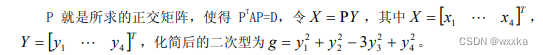
[p,d]=eig(a)
format short
p,d
% p =
%
% -1/2 390/1351 780/989 780/3691
% 1/2 -390/1351 780/3691 780/989
% 1/2 -390/1351 780/1351 -780/1351
% -1/2 -1170/1351 0 0
%
%
% d =
%
% -3 0 0 0
% 0 1 0 0
% 0 0 1 0
% 0 0 0 1
%
%
% p =
%
% -0.5000 0.2887 0.7887 0.2113
% 0.5000 -0.2887 0.2113 0.7887
% 0.5000 -0.2887 0.5774 -0.5774
% -0.5000 -0.8660 0 0
%
%
% d =
%
% -3.0000 0 0 0
% 0 1.0000 0 0
% 0 0 1.0000 0
% 0 0 0 1.0000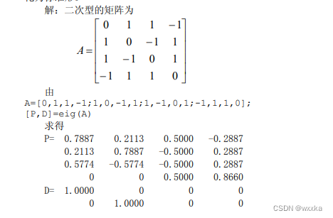

function test9_1
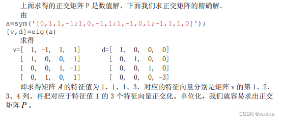
a=str2sym('[0 1 1 -1;1 0 -1 1;1 -1 0 1;-1 1 1 0]');
[p,d]=eig(a)
% p =
%
% [ 1, 1, 1, -1]
% [ -1, 1, 0, 0]
% [ -1, 0, 1, 0]
% [ 1, 0, 0, 1]
%
%
% d =
%
% [ -3, 0, 0, 0]
% [ 0, 1, 0, 0]
% [ 0, 0, 1, 0]
% [ 0, 0, 0, 1]
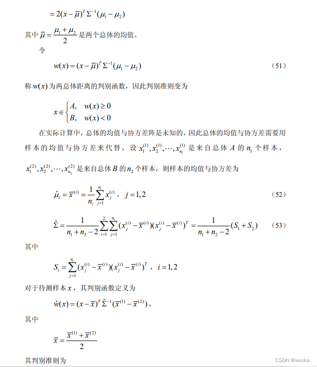
% 多元分析
综述:多元分析,是多变量统计分析方法。多变量统计分析的基本出发点:变量之间的相关性,不能简单地把每个变量结果进行汇总。
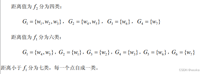
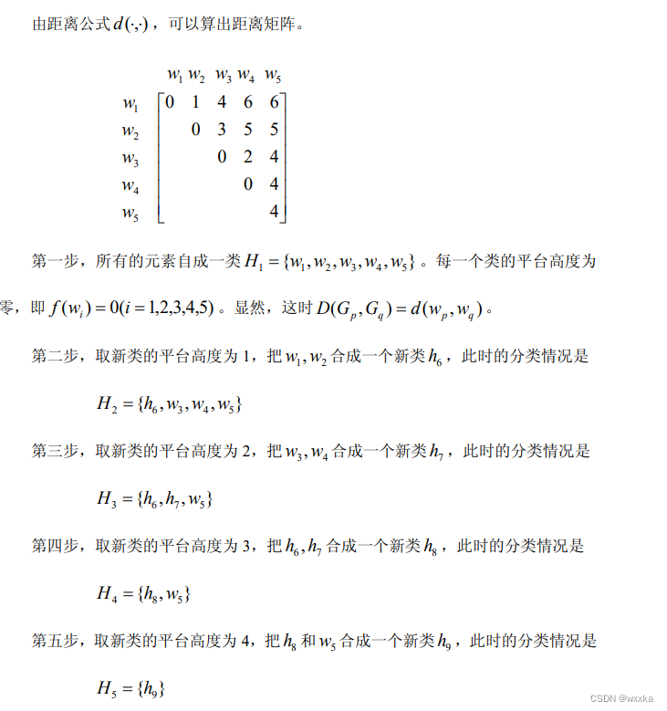
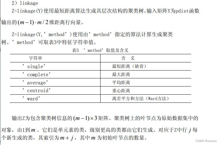
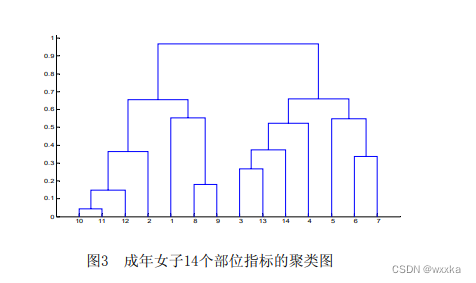
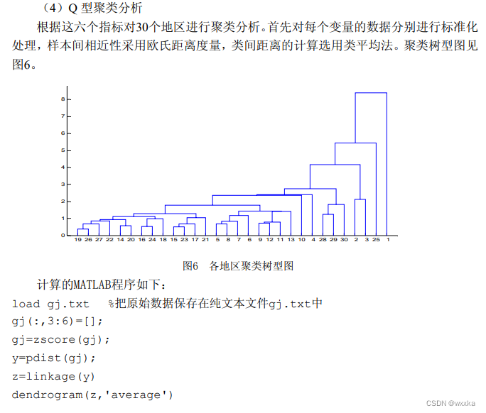
聚类分析
聚类分析,可以分为两类。一个是面对很多样本,如何将这些样本进行聚类分析,分几个类别,每个类别有不同的特点,这称为Q型聚类分析,就是样本聚类分析;另一个是,每个样本都有很多变量属性,这些属性并不是相互独立的,有的变量之间的相关性较强,即,有的变量可以归为一类,有的单独是一类,这是样本各个评价指标的变量分析,称为R型聚类分析。
聚类分析基本概念
相似性度量:
样本的相似性度量:样本有多个属性,每个属性可以视为一个坐标轴,那么含有n个属性的样本都能用n维空间中的一个点表示,这样,一个样本用一个点表示,自然而然,样本之间的相似性,可以用点与点之间的距离作为衡量。(从这里容易看出,对于样本的各个属性,要使用标准化或者归一化操作去除量纲,消除单位不同带来的影响,防止大数据吃掉小数据)下面给出距离的定义
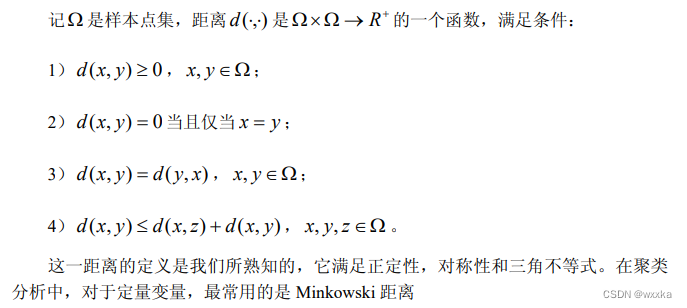
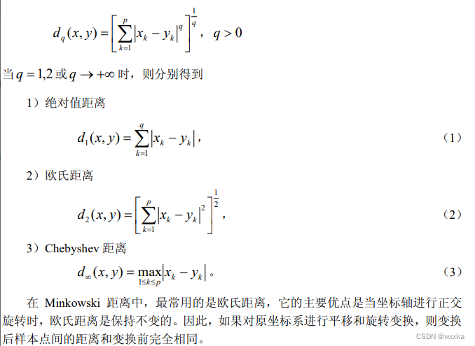
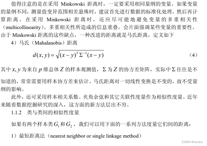
![]()
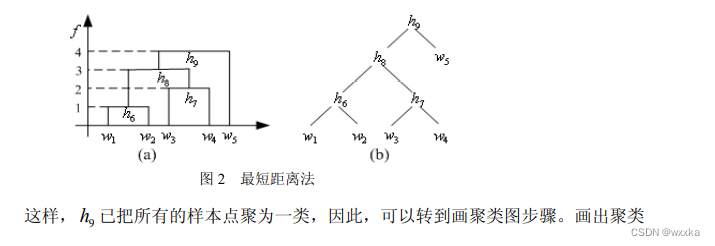
常用的有类平均法
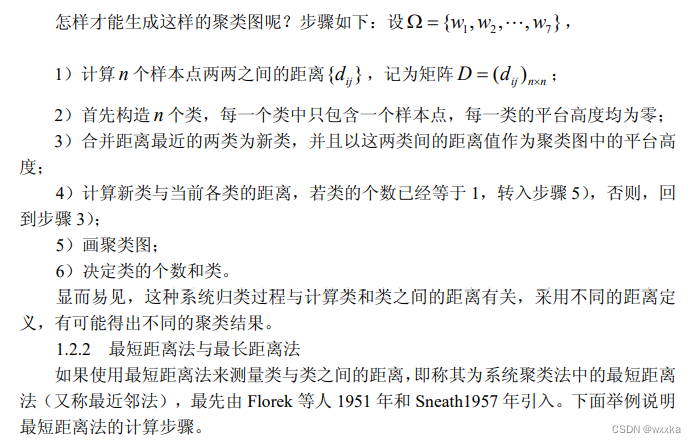
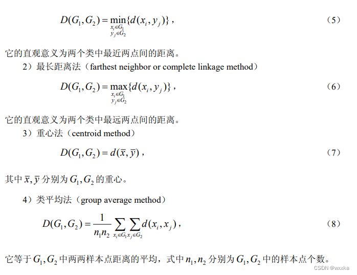
例题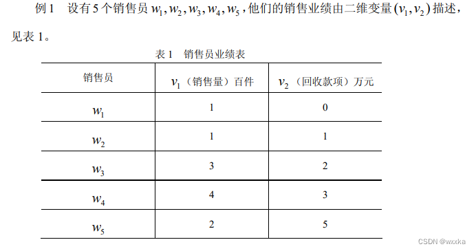
![]()
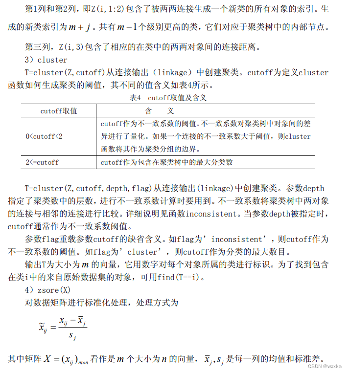

对样本的属性进行聚类分析,变量聚类法,R型聚类
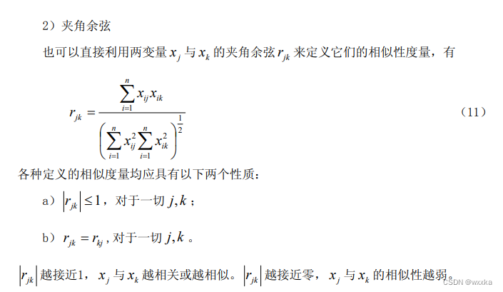
变量的相似性度量:相关系数,余弦夹角
变量聚类法:
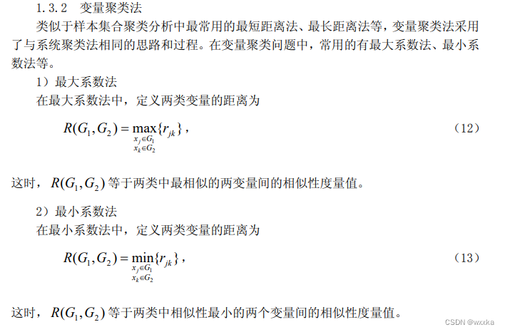
例子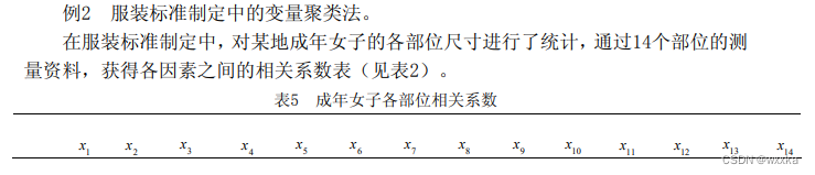
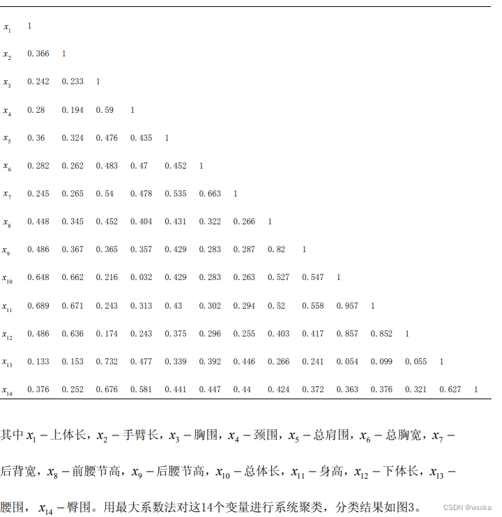
1
0.366	1
0.242	0.233	1
0.28	0.194	0.59	1
0.36	0.324	0.476	0.435	1
0.282	0.262	0.483	0.47	0.452	1
0.245	0.265	0.54	0.478	0.535	0.663	1
0.448	0.345	0.452	0.404	0.431	0.322	0.266	1
0.486	0.367	0.365	0.357	0.429	0.283	0.287	0.82	1
0.648	0.662	0.216	0.032	0.429	0.283	0.263	0.527	0.547	1
0.689	0.671	0.243	0.313	0.43	0.302	0.294	0.52	0.558	0.957	1
0.486	0.636	0.174	0.243	0.375	0.296	0.255	0.403	0.417	0.857	0.852	1
0.133	0.153	0.732	0.477	0.339	0.392	0.446	0.266	0.241	0.054	0.099	0.055	1
0.376	0.252	0.676	0.581	0.441	0.447	0.44	0.424	0.372	0.363	0.376	0.321	0.627	1
上面的数据文件名称edata10_2.txt;
clc, clear, close all
a=textread('data10_2.txt');%读取下三角相关系数
d=1-abs(a); %进行数据变换,把相关系数转化为距离
d=tril(d);  %提出d矩阵的下三角部分
b=nonzeros(d);%去掉d中的零元素
b=b';  %化成行向量
z=linkage(b,'complete'); %按最长距离法聚类
y=cluster(z,'maxclust',2)   %把变量划分成两类
ind1=find(y==1);ind1=ind1'  %显示第一类对应的变量标号
ind2=find(y==2);ind2=ind2'  %显示第二类对应的变量标号
figure
h=dendrogram(z); %画聚类图
set(h,'Color','k','LineWidth',1.3)  %把聚类图线的颜色改成黑色,线宽加粗

综合运用Q&&R聚类方法
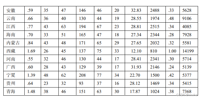
上面的数据,命名为anli10_1.txt
5.96 	310 	461 	1557 	931 	319 	44.36 	2615 	2.20 	13631
3.39 	234 	308 	1035 	498 	161 	35.02 	3052 	.90 	12665
2.35 	157 	229 	713 	295 	109 	38.40 	3031 	.86 	9385
1.35 	81 	111 	364 	150 	58 	30.45 	2699 	1.22 	7881
1.50 	88 	128 	421 	144 	58 	34.30 	2808 	.54 	7733
1.67 	86 	120 	370 	153 	58 	33.53 	2215 	.76 	7480
1.17 	63 	93 	296 	117 	44 	35.22 	2528 	.58 	8570
1.05 	67 	92 	297 	115 	43 	32.89 	2835 	.66 	7262
.95 	64 	94 	287 	102 	39 	31.54 	3008 	.39 	7786
.69 	39 	71 	205 	61 	24 	34.50 	2988 	.37 	11355
.56 	40 	57 	177 	61 	23 	32.62 	3149 	.55 	7693
.57 	58 	64 	181 	57 	22 	32.95 	3202 	.28 	6805
.71 	42 	62 	190 	66 	26 	28.13 	2657 	.73 	7282
.74 	42 	61 	194 	61 	24 	33.06 	2618 	.47 	6477
.86 	42 	71 	204 	66 	26 	29.94 	2363 	.25 	7704
1.29 	47 	73 	265 	114 	46 	25.93 	2060 	.37 	5719
1.04 	53 	71 	218 	63 	26 	29.01 	2099 	.29 	7106
.85 	53 	65 	218 	76 	30 	25.63 	2555 	.43 	5580
.81 	43 	66 	188 	61 	23 	29.82 	2313 	.31 	5704
.59 	35 	47 	146 	46 	20 	32.83 	2488 	.33 	5628
.66 	36 	40 	130 	44 	19 	28.55 	1974 	.48 	9106
.77 	43 	63 	194 	67 	23 	28.81 	2515 	.34 	4085
.70 	33 	51 	165 	47 	18 	27.34 	2344 	.28 	7928
.84 	43 	48 	171 	65 	29 	27.65 	2032 	.32 	5581
1.69 	26 	45 	137 	75 	33 	12.10 	810 	1.00 	14199
.55 	32 	46 	130 	44 	17 	28.41 	2341 	.30 	5714
.60 	28 	43 	129 	39 	17 	31.93 	2146 	.24 	5139
1.39 	48	62 	208	77 	34	22.70 	1500 	.42 	5377
.64 	23 	32 	93 	37 	16 	28.12 	1469	.34	5415
1.48 	38 	46 	151 	63 	30 	17.87 	1024 	.38 	7368
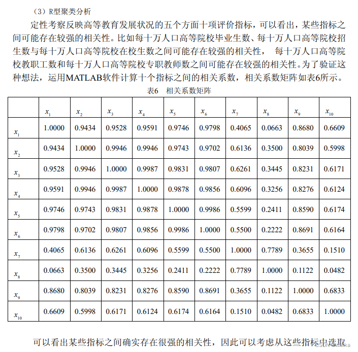
R型聚类分析---分析样本所含变量之间的相关性,避免多重线性性对分析的影响
%%
%变量聚类 R-聚类
%% 第一种聚类方法
clc, clear, close all
%a=readmatrix('anli10_1.txt');
a=load('anli10_1.txt');

b=zscore(a); %数据标准化%去除量纲影响
%对每一列进行标准化(每一列表示的是相同的属性)
% Z = zscore(X) returns the z-score for each element
%of X such that columns of X are centered to have
%mean 0 and scaled to have standard deviation 1.
%Z is the same size as X.
% If X is a vector, then Z is a vector of z-scores.
% If X is a matrix, then Z is a matrix of
%the same size as X, and each column of Z has mean 0
%and standard deviation 1.

z=linkage(b','average','correlation');  %按类平均法聚类
figure
h=dendrogram(z);  %画聚类图
set(h,'Color','k','LineWidth',1.3)  %把聚类图线的颜色改成黑色,线宽加粗
T=cluster(z,'maxclust',6)  %把变量划分成6类
for i=1:6
    tm=find(T==i);  %求第i类的对象
    fprintf('第%d类的有%s\n',i,int2str(tm')); %显示分类结果
end


%% 采用另一种聚类度量方法--相关系数距离
clc, clear, close all
%a=readmatrix('anli10_1.txt');
a=load('anli10_1.txt');
b=zscore(a); %数据标准化%去除量纲影响

r=corrcoef(b) %计算相关系数矩阵
%r=corrcoef(b)输入矩阵b,n*m,n个样本的m个属性矩阵
%%输入的b每一列表示同一个属性
%输出r是m*m矩阵,表示列与列之间的相关系数,
%即每个属性之间相关系数
% %corrcoef示例
% x = randn(6,1);
% y = randn(6,1);
% A = [x y 2*y+3];
% R = corrcoef(A)

d=tril(1-r); d=nonzeros(d); %另外一种计算距离方法
z=linkage(d');  %按类平均法聚类
figure
h=dendrogram(z);  %画聚类图
set(h,'Color','k','LineWidth',1.3)  %把聚类图线的颜色改成黑色,线宽加粗
T=cluster(z,'maxclust',6)  %把变量划分成6类
for i=1:6
    tm=find(T==i);  %求第i类的对象
    fprintf('第%d类的有%s\n',i,int2str(tm')); %显示分类结果
end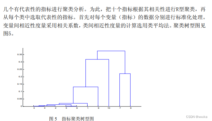
下面,紧接着,进行样本聚类分析,即Q型聚类分析
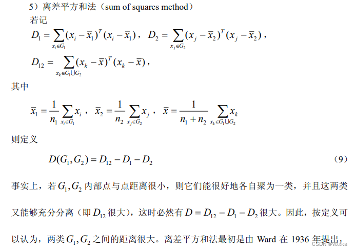
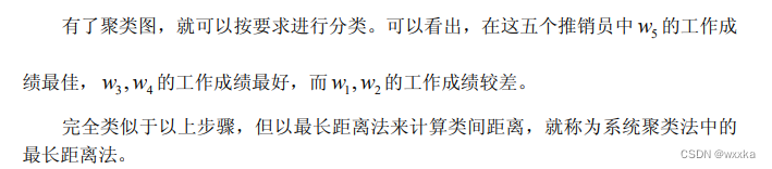
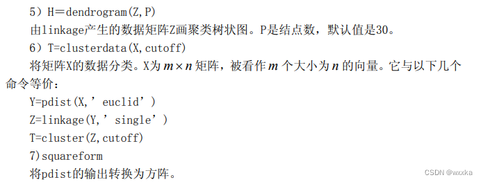
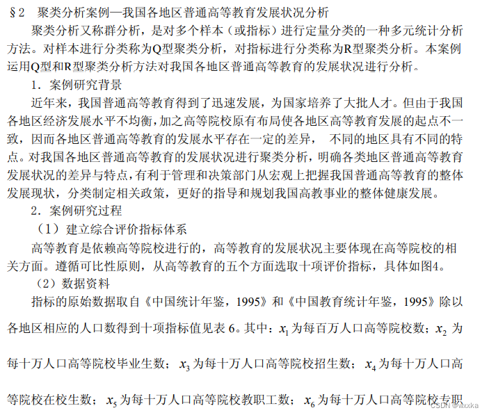
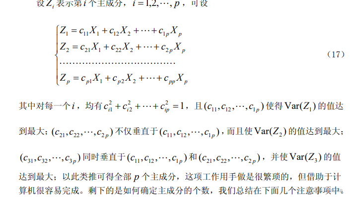
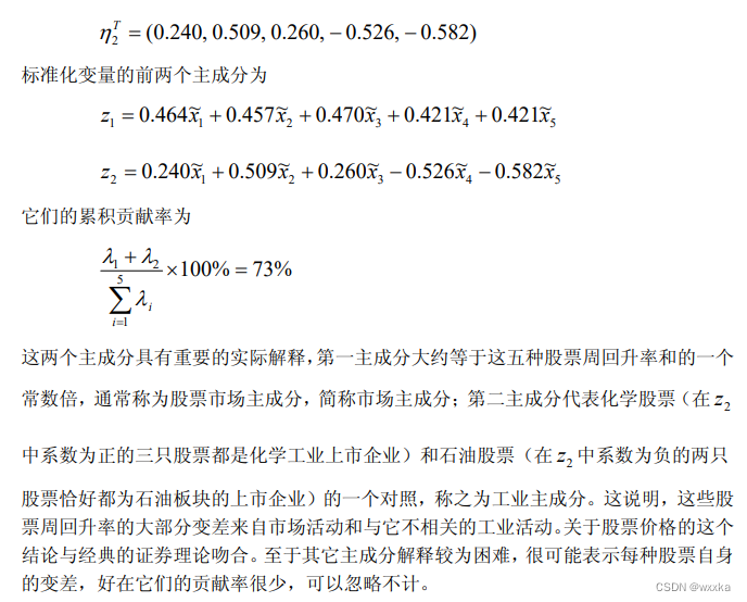
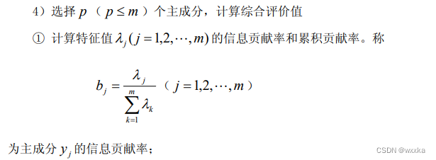
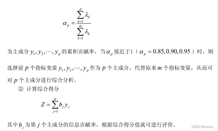
主成分分析
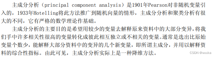
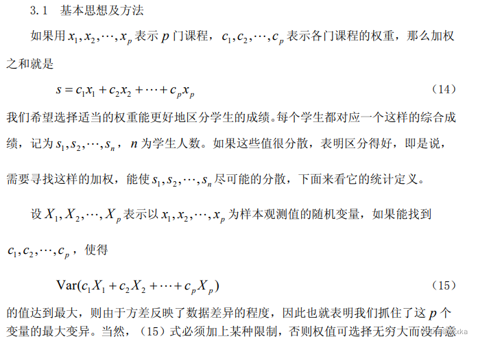
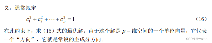

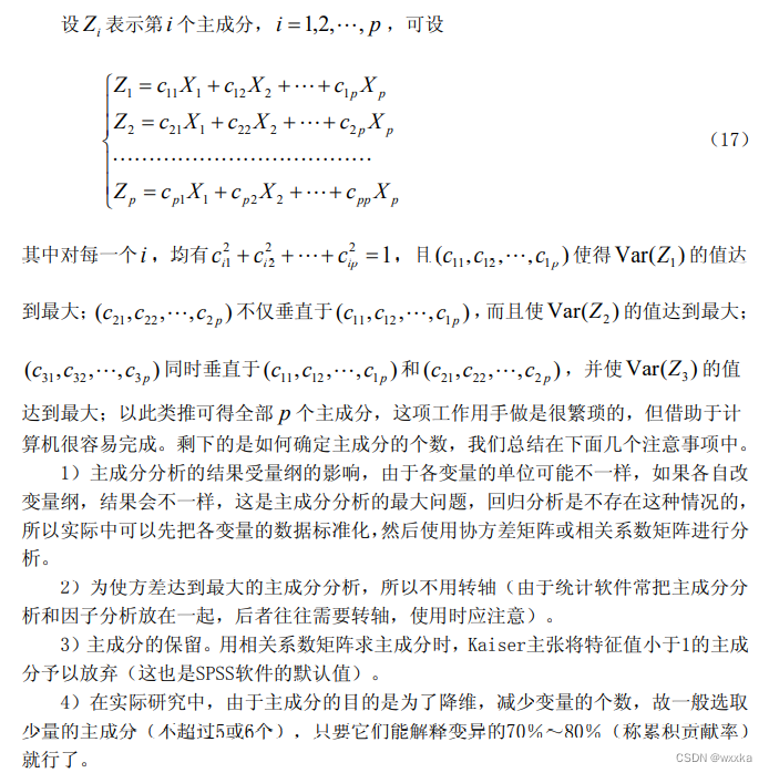
主成分分析,利用已知的m维属性的样本数据X,找到m维方向向量C,时X*C的方差最大(差异化最大,方差表示差异化,方差越大,差异化越大,差异越大,表明找到了已知的m维变量的最大变异),单位化使求得的结果C有意义。
由上,求得的便叫作主成分。一般,求一个主成分不够,还要求几个,并且保证求得的主成分互相正交(这是m维空间,必能求到m个互相正交的单位向量)
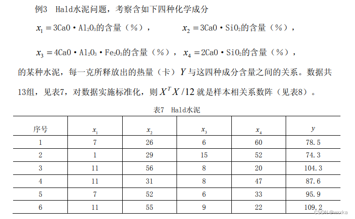
数据data10_5.txt
7 26 6 60 78.5
1 29 15 52 74.3
11 56 8 20 104.3
11 31 8 47 87.6
7 52 6 33 95.9
11 55 9 22 109.2
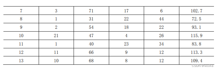
3 71 17 6 102.7
1 31 22 44 72.5
2 54 18 22 93.1
21 47 4 26 115.9
1 40 23 34 83.8
11 66 9 12 113.3
10 68 8 12 109.4
![]()
代码如下
clc,clear
%a=readmatrix('data10_5.txt');
a=load('data10_5.txt');
[m,n]=size(a);
x0=a(:,[1:n-1]); y0=a(:,n);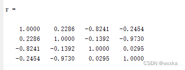
r=corrcoef(x0) %计算相关系数矩阵 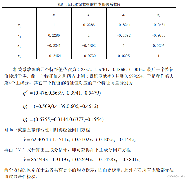
clc,clear
%输入数据
a=load('data10_5.txt');
[m,n]=size(a);
x0=a(:,[1:n-1]); y0=a(:,n);
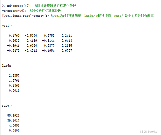
xd=zscore(x0); %对设计矩阵进行标准化处理
yd=zscore(y0); %对y0进行标准化处理
r=corrcoef(x0) %计算相关系数矩阵
%% 直接做最小二乘法线性回归
%左除计算回归系数%线性%下面的左除自带的是最小二乘法
hg1=[ones(m,1),x0]\y0; %计算普通最小二乘法回归系数
%变成行向量显示回归系数,其中第1个分量是常数项,
%其它按x1,...,xn排序
hg1=hg1'
%输出最小二乘法结果结果
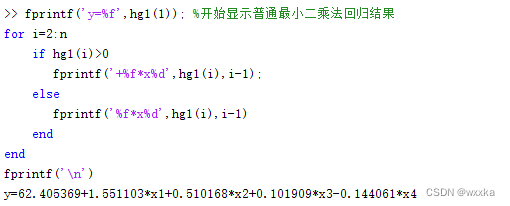
fprintf('y=%f',hg1(1)); %开始显示普通最小二乘法回归结果
for i=2:n
if hg1(i)>0
fprintf('+%f*x%d',hg1(i),i-1);
else
fprintf('%f*x%d',hg1(i),i-1)
end
end
fprintf('\n')
%% 最小二乘法+pca主成分分析回归
xd=zscore(x0); %对设计矩阵进行标准化处理
yd=zscore(y0); %对y0进行标准化处理
[vec1,lamda,rate]=pcacov(r) %vec1为r的特征向量,lamda为r的特征值,rate为各个主成分的贡献率
f=repmat(sign(sum(vec1)),size(vec1,1),1); %构造与vec1同维数的元素为±1的矩阵
vec2=vec1.*f %修改特征向量的正负号,使得特征向量的所有分量和为正
contr=cumsum(rate) %计算累积贡献率,第i个分量表示前i个主成分的贡献率%根据这个,确定主成分个数是3
df=xd*vec2; %计算所有主成分的得分
num=input('请选项主成分的个数:') %通过累积贡献率交互式选择主成分的个数%输入3
hg21=df(:,[1:num])\yd %主成分变量的回归系数,这里由于数据标准化,回归方程的常数项为0
hg22=vec2(:,1:num)*hg21 %标准化变量的回归方程系数
hg23=[mean(y0)-std(y0)*mean(x0)./std(x0)*hg22, std(y0)*hg22'./std(x0)] %计算原始变量回归方程的系数
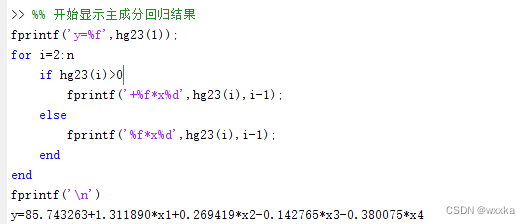
%% 开始显示主成分回归结果
fprintf('y=%f',hg23(1));
for i=2:n
if hg23(i)>0
fprintf('+%f*x%d',hg23(i),i-1);
else
fprintf('%f*x%d',hg23(i),i-1);
end
end
fprintf('\n')
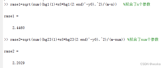
%% 下面计算两种回归分析的剩余标准差
rmse1=sqrt(sum((hg1(1)+x0*hg1(2:end)'-y0).^2)/(m-n)) %拟合了n个参数
rmse2=sqrt(sum((hg23(1)+x0*hg23(2:end)'-y0).^2)/(m-num)) %拟合了num个参数
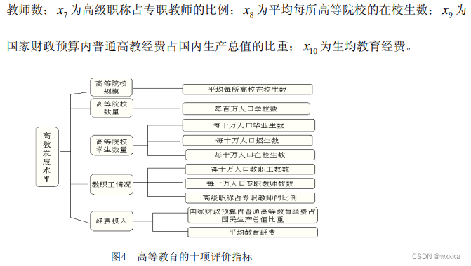
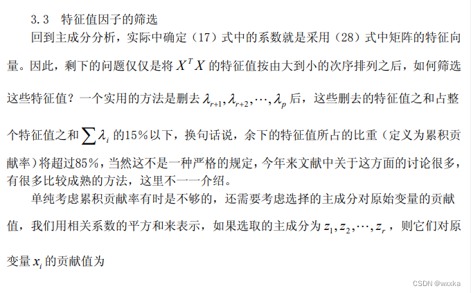
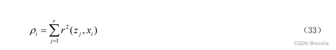
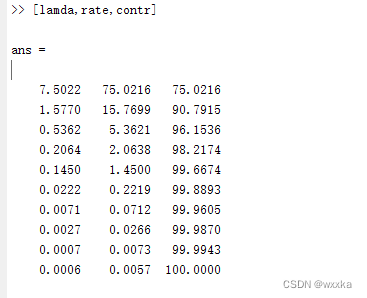
显著性检验---置信区间--置信度
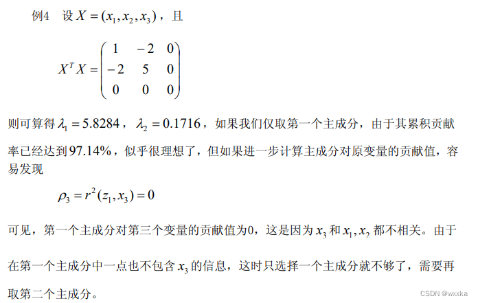
确定特征成分个数:1.累计贡献率2.选择的主成分对原始变量的贡献值---相关系数
![]()

输入数据--》标准化--》相关系数作为变量相似性度量--》pca主成分提取

原始数据文件见上
clc, clear, close all
%a=readmatrix('anli10_1.txt');
a=load('anli10_1.txt');
a=zscore(a);
r=corrcoef(a)
[vec1,lamda,rate]=pcacov(r) %vec1为r的特征向量,lamda为r的特征值,rate为各个主成分的贡献率
f=repmat(sign(sum(vec1)),size(vec1,1),1); %构造与vec1同维数的元素为±1的矩阵
vec2=vec1.*f %修改特征向量的正负号,使得特征向量的所有分量和为正
contr=cumsum(rate) %计算累积贡献率,第i个分量表示前i个主成分的贡献率
%根据这个,确定主成分个数是4
%每个主成分占一列
% df=a*vec2;  %计算所有主成分的得分
vec1(:,1:4)
df=a*vec2(:,1:4);  %计算前四个主成分的得分
tf=df*rate(1:4)/100
[stf,ind]=sort(tf,'descend')
[stf,ind]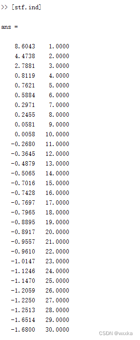
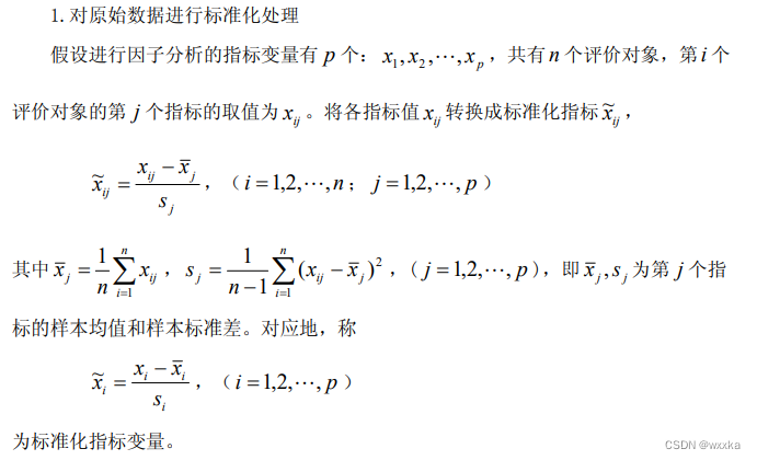
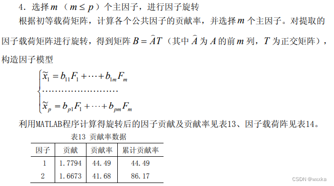
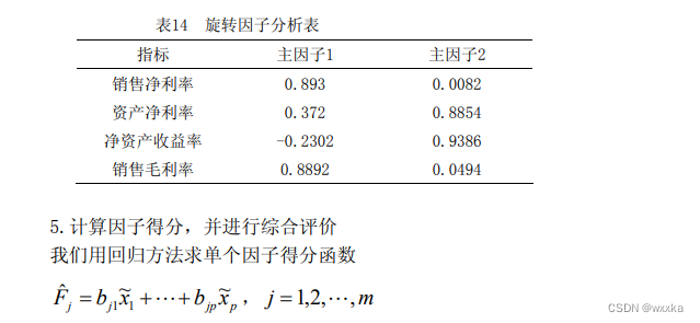
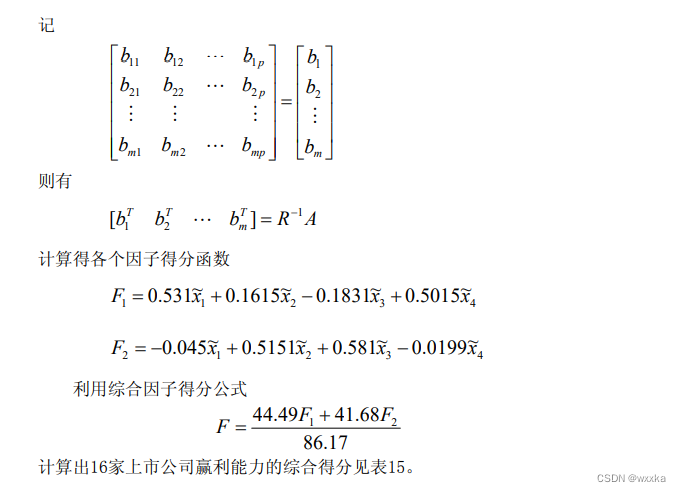
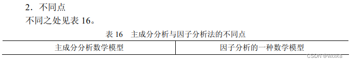
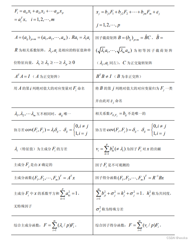
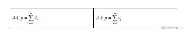
因子分析
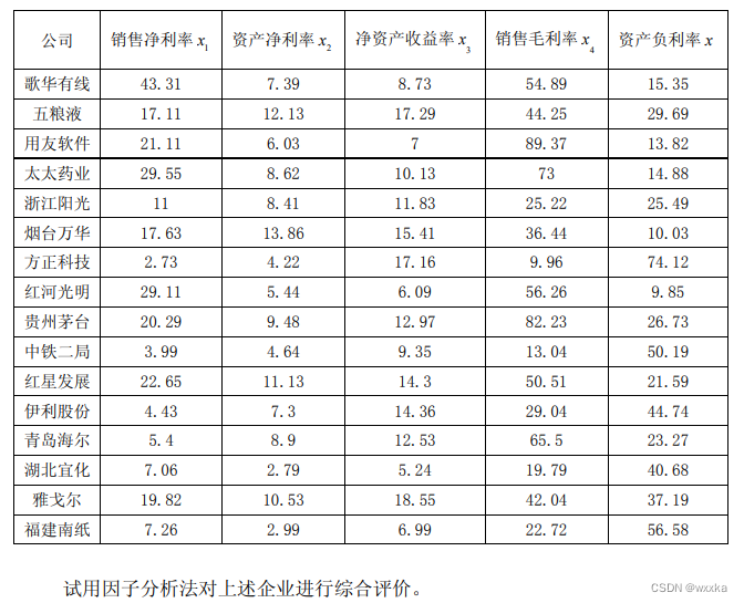
数据文件anli10_3.txt
43.31	7.39	8.73	54.89	15.35
17.11	12.13	17.29	44.25	29.69
21.11	6.03	7	89.37	13.82
29.55	8.62	10.13	73	14.88
11	8.41	11.83	25.22	25.49
17.63	13.86	15.41	36.44	10.03
2.73	4.22	17.16	9.96	74.12
29.11	5.44	6.09	56.26	9.85
20.29	9.48	12.97	82.23	26.73
3.99	4.64	9.35	13.04	50.19
22.65	11.13	14.3	50.51	21.59
4.43	7.3	14.36	29.04	44.74
5.4	8.9	12.53	65.5	23.27
7.06	2.79	5.24	19.79	40.68
19.82	10.53	18.55	42.04	37.19
7.26	2.99	6.99	22.72	56.58
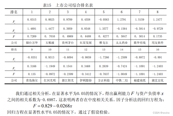
得分和负债水平的相关系数和对应置信水平
得分与负债水平的回归方程及对应显著水平
clear
%% 0%导入数据
a = load('anli10_3.txt');
n=size(a,1);%获得样本个数
x=a(:,[1:4]); y=a(:,5); %分别提出自变量x1...x4和因变量y的值
%% 1标准化
x=zscore(x); %数据标准化
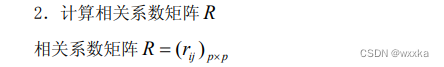
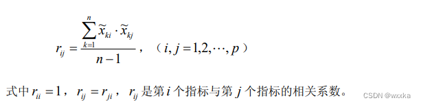
%% 2计算相关系数矩阵
r=corrcoef(x) %求相关系数矩阵
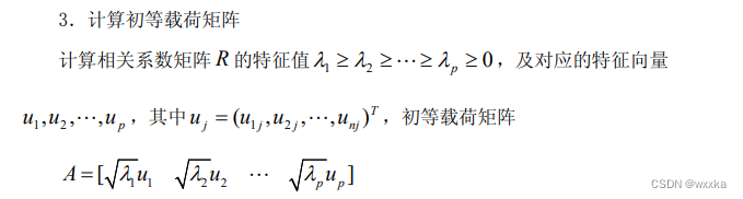
%% 3%计算初等载荷矩阵
%计算相关系数矩阵的特征值和对应特征向量
%vel是特征向量,val是特征值,con1是贡献率
[vec1,val,con1]=pcacov(r) %进行主成分分析的相关计算
f1=repmat(sign(sum(vec1)),size(vec1,1),1);
vec2=vec1.*f1; %特征向量正负号转换
f2=repmat(sqrt(val)',size(vec2,1),1);
a=vec2.*f2 %求初等载荷矩阵
%factoran computes the maximum likelihood
%estimate (MLE) of the factor loadings matrix Λ
%in the factor analysis model
%x=μ+Λf+e
%如果指标变量多,选取的主因子个数少,
%可以直接使用factoran进行因子分析
%% 4选择初等载荷矩阵
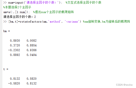
%num=input('请选择主因子的个数:'); %交互式选择主因子的个数
num=2;
%本题选择2个主因子
am=a(:,[1:num]); %提出num个主因子的载荷矩阵
[bm,t]=rotatefactors(am,'method', 'varimax') %am旋转变换,bm为旋转后的载荷阵
bt=[bm,a(:,[num+1:end])]; %旋转后的载荷阵,前两个旋转,后面不旋转
con2=sum(bt.^2) %计算因子贡献
check=[con1,con2'/sum(con2)*100] %未旋转和旋转后的贡献率对照
rate=con2(1:num)/sum(con2) %计算因子贡献率
con=cumsum(rate)
%贡献-贡献率-累计贡献率%贡献率数据
[con2(1:num)',rate',con']
%% 计算因子得分,进行综合评价
coef=inv(r)*bm %计算得分函数的系数
score=x*coef %计算各个因子的得分
weight=rate/sum(rate) %计算得分的权重
Tscore=score*weight' %对各因子的得分进行加权求和,即求各企业综合得分
[STscore,ind]=sort(Tscore,'descend') %对企业进行排序%得分F
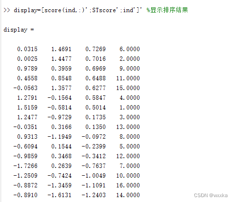
display=[score(ind,:)';STscore';ind']' %显示排序结果
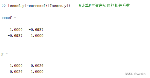
[ccoef,p]=corrcoef([Tscore,y]) %计算F与资产负债的相关系数
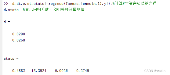
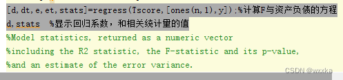
[d,dt,e,et,stats]=regress(Tscore,[ones(n,1),y]);%计算F与资产负债的方程
d,stats %显示回归系数,和相关统计量的值
%Model statistics, returned as a numeric vector
%including the R2 statistic, the F-statistic and its p-value,
%and an estimate of the error variance.
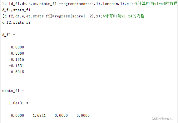
%% 利用regress求解线性回归方程
%计算F1与x1-x4的方程
[d_f1,dt,e,et,stats_f1]=regress(score(:,1),[ones(n,1),x]);
d_f1,stats_f1
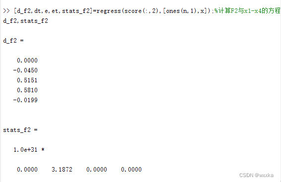
%计算F2与x1-x4的方程
[d_f2,dt,e,et,stats_f2]=regress(score(:,2),[ones(n,1),x]);
d_f2,stats_f2
% format short
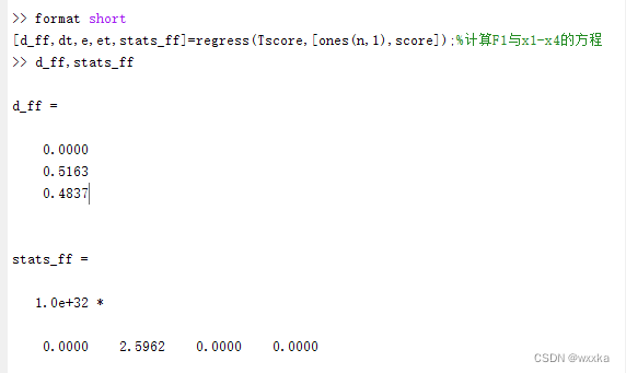
%计算F与F1/F2的方程
[d_ff,dt,e,et,stats_ff]=regress(Tscore,[ones(n,1),score]);
d_ff,stats_ff 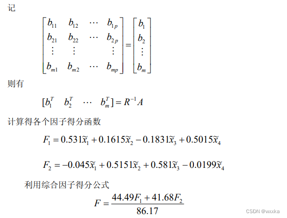

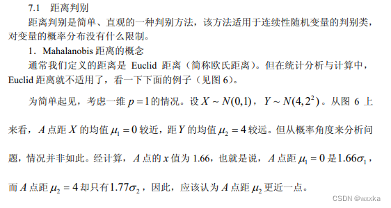
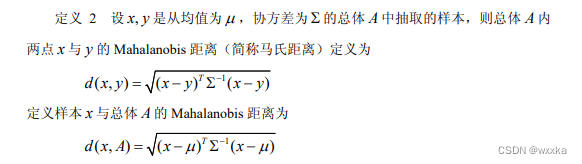
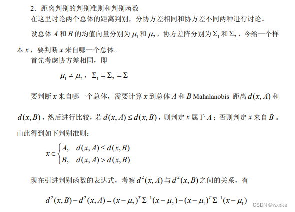
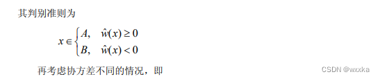
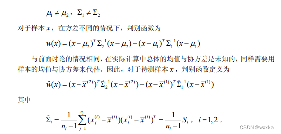
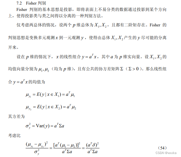
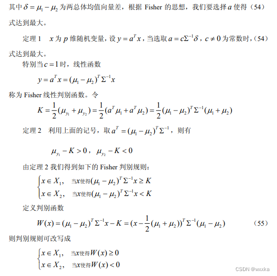
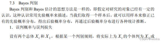
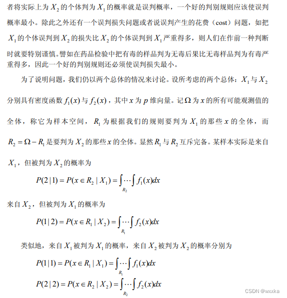
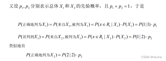
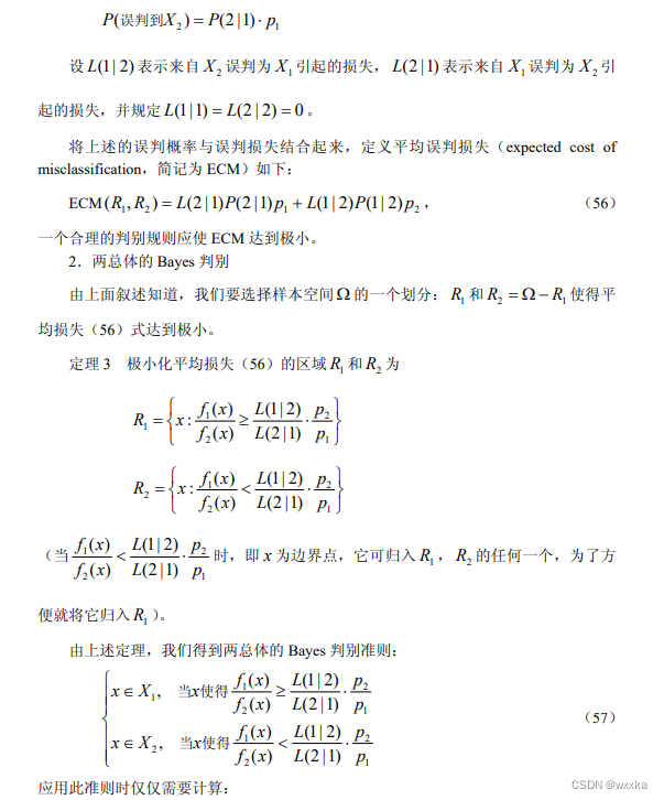
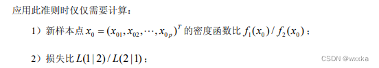
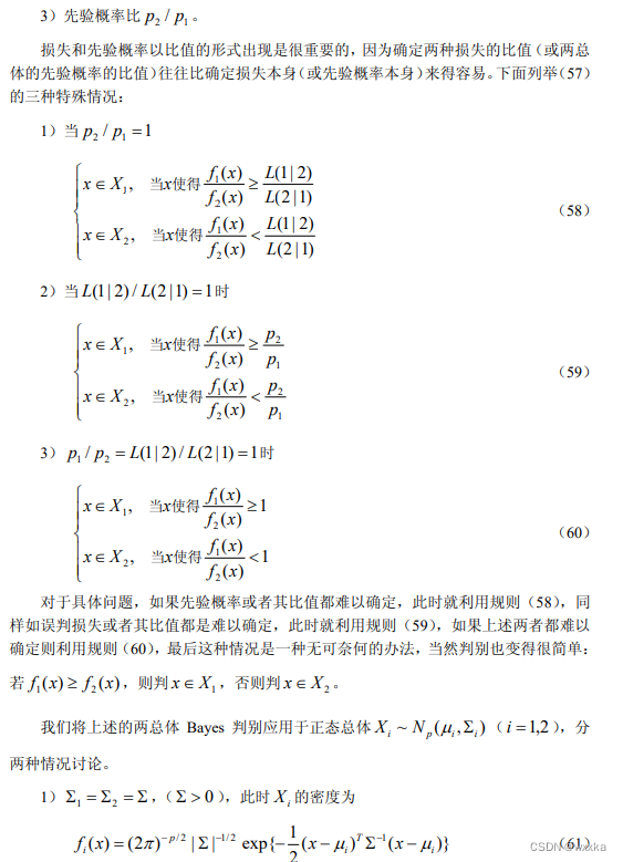
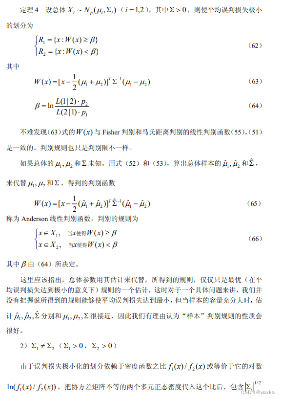
判别分析
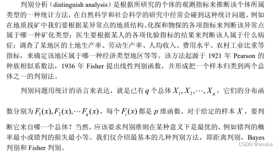
判别分析,根据样本的属性,推断样本的类别,类似于无监督分类模型


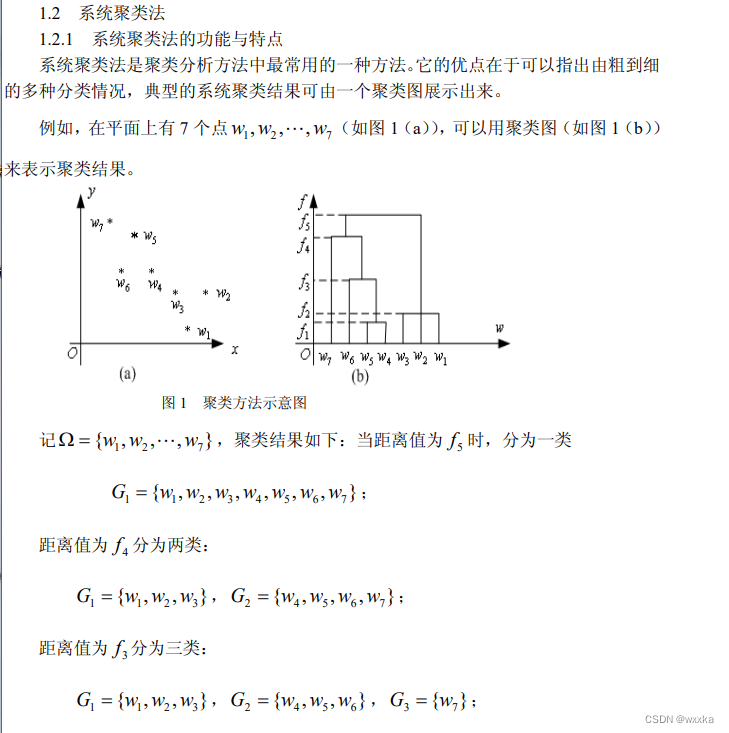
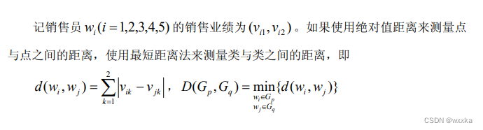
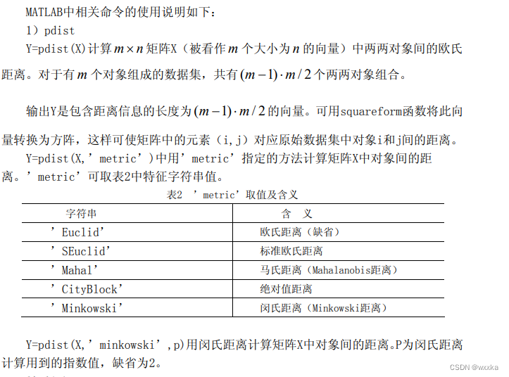
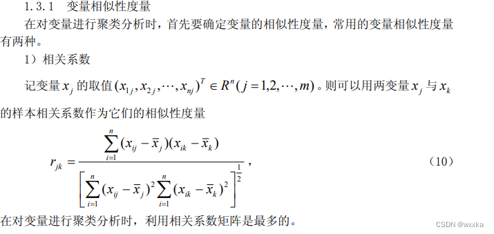
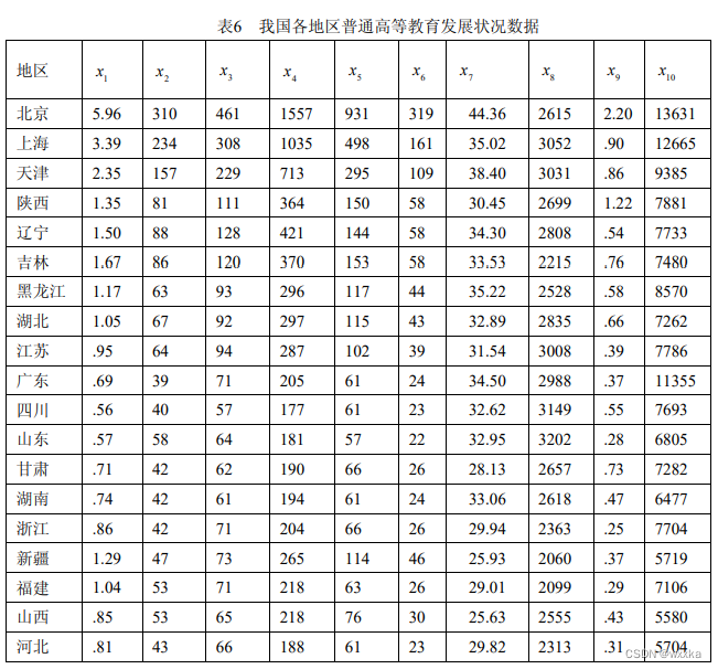
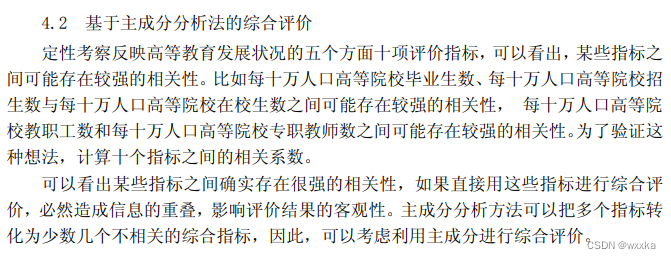
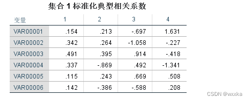
典型相关性分析

![]()
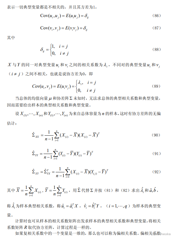
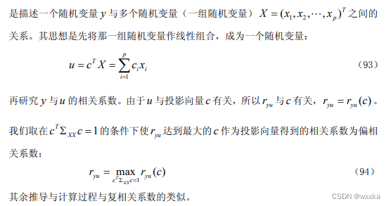
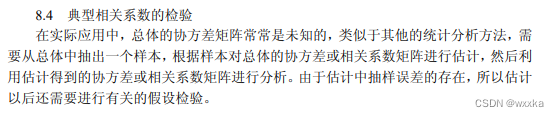
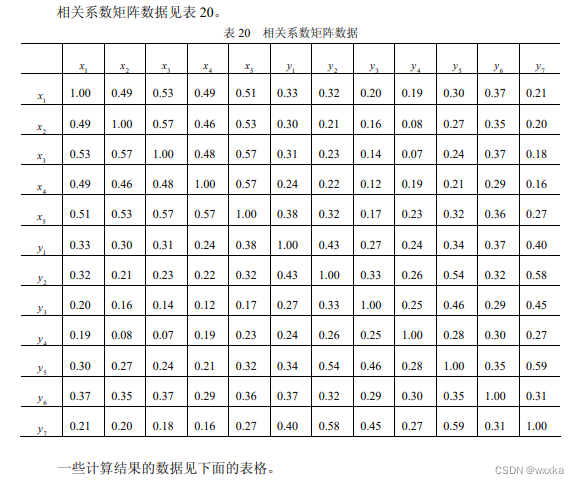
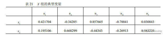
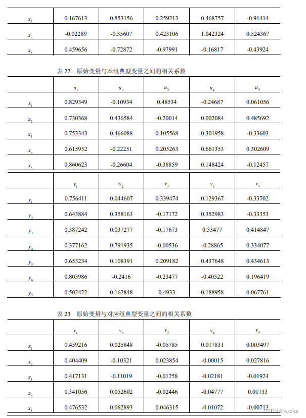
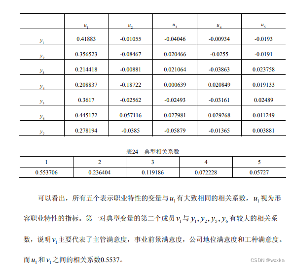
从表24知,u和v之间的相关系数是0.5537
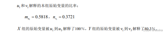
如上,得到u和v解释本组原始变量的比率分别是0.5818、0.3721
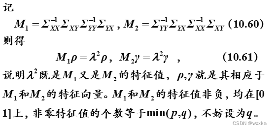
表2-1
典型相关系数
x-u,y-v
x-v,y-u相关系数
anli10_5_1.txt
1.00	0.49	0.53	0.49	0.51	0.33	0.32	0.20	0.19	0.30	0.37	0.21
0.49	1.00	0.57	0.46	0.53	0.30	0.21	0.16	0.08	0.27	0.35	0.20
0.53	0.57	1.00	0.48	0.57	0.31	0.23	0.14	0.07	0.24	0.37	0.18
0.49	0.46	0.48	1.00	0.57	0.24	0.22	0.12	0.19	0.21	0.29	0.16
0.51	0.53	0.57	0.57	1.00	0.38	0.32	0.17	0.23	0.32	0.36	0.27
0.33	0.30	0.31	0.24	0.38	1.00	0.43	0.27	0.24	0.34	0.37	0.40
0.32	0.21	0.23	0.22	0.32	0.43	1.00	0.33	0.26	0.54	0.32	0.58
0.20	0.16	0.14	0.12	0.17	0.27	0.33	1.00	0.25	0.46	0.29	0.45
0.19	0.08	0.07	0.19	0.23	0.24	0.26	0.25	1.00	0.28	0.30	0.27
0.30	0.27	0.24	0.21	0.32	0.34	0.54	0.46	0.28	1.00	0.35	0.59
0.37	0.35	0.37	0.29	0.36	0.37	0.32	0.29	0.30	0.35	1.00	0.31
0.21	0.20	0.18	0.16	0.27	0.40	0.58	0.45	0.27	0.59	0.31	1.00
function anli10_5_fuben
clear
%% 数据导入
r = load('anli10_5_1.txt'); %读入相关系数矩阵
%% 根据公式(81)求m1和m2
n1=5; n2=7; num=min(n1,n2);
s11=r([1:n1],[1:n1]); %提出X与X的相关系数
s12=r([1:n1],[n1+1:end]); %提出X与Y的相关系数
s21=s12'; %提出Y与X的相关系数
s22=r([n1+1:end],[n1+1:end]); %提出Y与Y的相关系数
m1=inv(s11)*s12*inv(s22)*s21; %计算矩阵M1,式(81)
m2=inv(s22)*s21*inv(s11)*s12; %计算矩阵M2,式(81)
%% 求m1、m2特征值特征向量
[vec1,val1]=eig(m1); %求M1的特征向量vec1和特征值val1
for i=1:n1
vec1(:,i)=vec1(:,i)/sqrt(vec1(:,i)'*s11*vec1(:,i));
%特征向量归一化,满足a's1a=1
vec1(:,i)=vec1(:,i)*sign(sum(vec1(:,i)));
%特征向量乘以1或-1,保证所有分量和为正
end
val1=sqrt(diag(val1)); %计算特征值的平方根
[val1,ind1]=sort(val1,'descend'); %按照从大到小排列
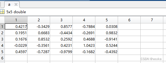
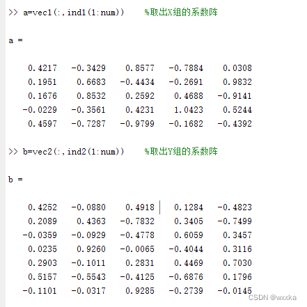
a=vec1(:,ind1(1:num)) %取出X组的系数阵
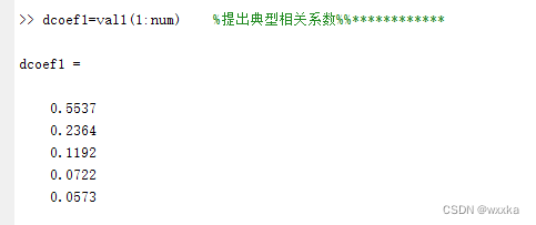
% 典型相关系数
dcoef1=val1(1:num) %提出典型相关系数%%************
[vec2,val2]=eig(m2);
for i=1:n2
vec2(:,i)=vec2(:,i)/sqrt(vec2(:,i)'*s22*vec2(:,i));
vec2(:,i)=vec2(:,i)*sign(sum(vec2(:,i)));
end
val2=sqrt(diag(val2)); %计算特征值的平方根
[val2,ind2]=sort(val2,'descend'); %按照从大到小排列
b=vec2(:,ind2(1:num)) %取出Y组的系数阵
% 典型相关系数
dcoef2=val2(1:num) %提出典型相关系数
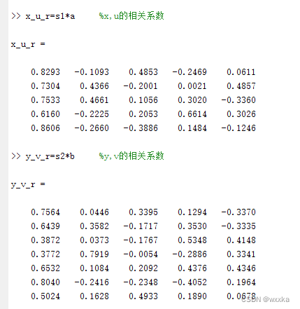
%% x/y与u、v之间的相关系数
x_u_r=s11*a %x,u的相关系数
y_v_r=s22*b %y,v的相关系数
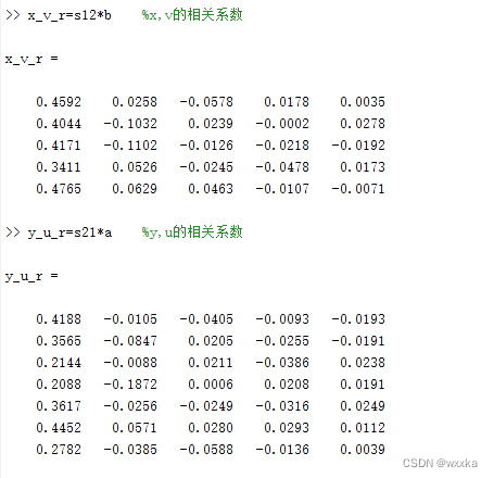
x_v_r=s12*b %x,v的相关系数
y_u_r=s21*a %y,u的相关系数
%% u和v分别解释x、y的比率
%u解释x组变量--v解释y组变量
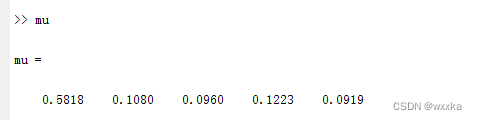
mu=sum(x_u_r.^2)/n1 %x组原始变量被u_i解释的方差比例
mv=sum(x_v_r.^2)/n1 %x组原始变量被v_i解释的方差比例%sum(mv)
nu=sum(y_u_r.^2)/n2 %y组原始变量被u_i解释的方差比例%sum(nu)
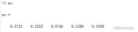
nv=sum(y_v_r.^2)/n2 %y组原始变量被v_i解释的方差比例
fprintf('X组的原始变量被u1~u%d解释的比例为%f\n',num,sum(mu));
fprintf('Y组的原始变量被v1~v%d解释的比例为%f\n',num,sum(nv));

典型相关性分析步骤
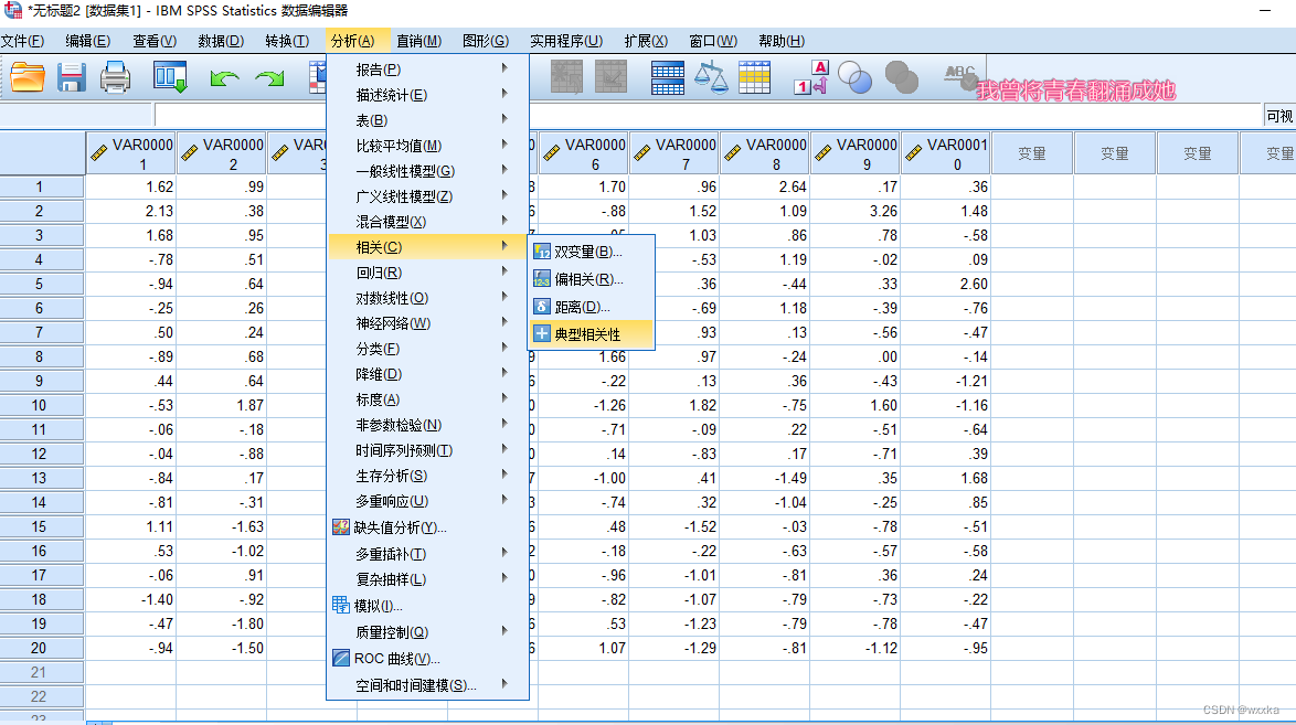
matlab求解,u=u(x1,x2,x3,x4,x5,x6) ,u=(u1,u2)
v=v(y1,y2,y3,y4),v=(v1,v2)
clear
%导入数据
load x
load y
%数据预处理
p=size(x,2);q=size(y,2);
x=zscore(x);y=zscore(y); %标准化数据
n=size(x,1); %观测数据的个数
%下面做典型相关分析
%a1,b1返回的是典型变量的系数,
%r返回的是典型相关系数
%u1,v1返回的是典型变量的值,
%stats返回的是假设检验的一些统计量的值
[a1,b1,r,u1,v1,stats]=canoncorr(x,y)
%根据上面输出的stats,判断怎么利用获得的a1、b1、u1、v1的值,
%下面修正a1,b1每一列的正负号,使得a,b每一列的系数和为正
%对应的,典型变量取值的正负号也要修正
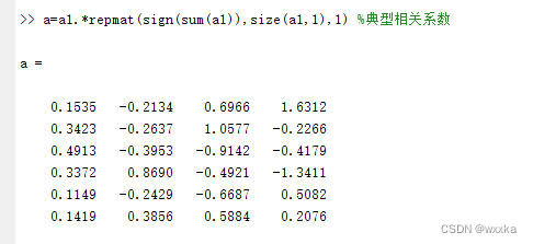
a=a1.*repmat(sign(sum(a1)),size(a1,1),1) %集合1典型标准化相关系数%u=u(x1,x2,x3,x4,x5,x6)
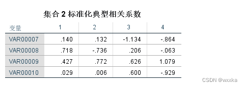
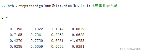
b=b1.*repmat(sign(sum(b1)),size(b1,1),1) %集合2典型相关系数
u=u1.*repmat(sign(sum(a1)),size(u1,1),1)
v=v1.*repmat(sign(sum(b1)),size(v1,1),1)
%% 计算x/y与u/v之间的相关系数
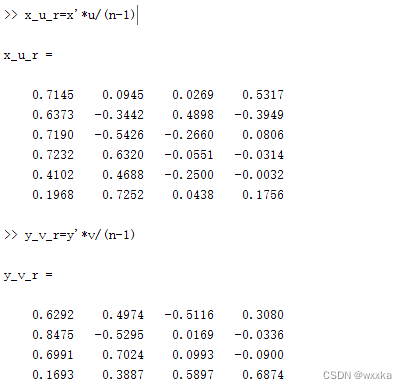
x_u_r=x'*u/(n-1) %计算x,u的相关系数%集合1典型载荷
y_v_r=y'*v/(n-1) %计算y,v的相关系数%集合2典型载荷
x_v_r=x'*v/(n-1) %计算x,v的相关系数%集合1交叉载荷
y_u_r=y'*u/(n-1) %计算y,u的相关系数%集合2交叉载荷
%% 典型相关系数的平方
val=r.^2 %典型相关系数的平方,M1或M2矩阵的非零特征值
%% x组原始变量
ux=sum(x_u_r.^2)/p %x组原始变量被u_i解释的方差比例
ux_cum=cumsum(ux) %x组原始变量被u_i解释的方差累积比例
vx=sum(x_v_r.^2)/p %x组原始变量被v_i解释的方差比例
vx_cum=cumsum(vx) %x组原始变量被v_i解释的方差累积比例
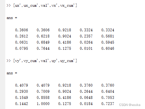
[ux',ux_cum',val',vx',vx_cum']
%% y组原始变量
vy=sum(y_v_r.^2)/q %y组原始变量被v_i解释的方差比例
vy_cum=cumsum(vy) %y组原始变量被v_i解释的方差累积比例
uy=sum(y_u_r.^2)/q %y组原始变量被u_i解释的方差比例
uy_cum=cumsum(uy) %y组原始变量被u_i解释的方差累积比例
[vy',vy_cum',val',uy',uy_cum']

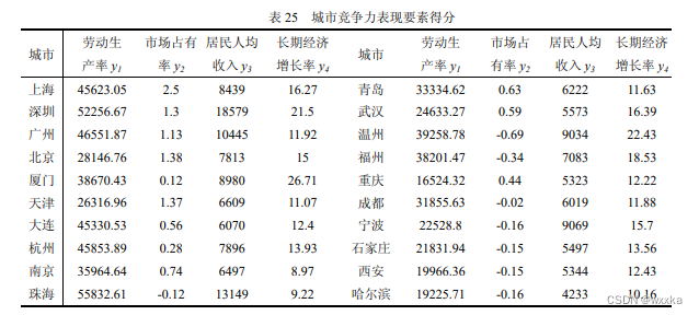
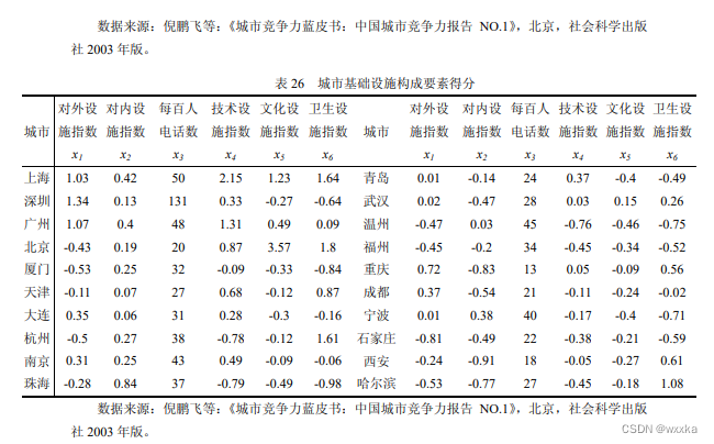
x.txt
1.03	0.42	50	2.15	1.23	1.64
1.34	0.13	131	0.33	-0.27	-0.64
1.07	0.4	48	1.31	0.49	0.09
-0.43	0.19	20	0.87	3.57	1.8
-0.53	0.25	32	-0.09	-0.33	-0.84
-0.11	0.07	27	0.68	-0.12	0.87
0.35	0.06	31	0.28	-0.3	-0.16
-0.5	0.27	38	-0.78	-0.12	1.61
0.31	0.25	43	0.49	-0.09	-0.06
-0.28	0.84	37	-0.79	-0.49	-0.98
0.01	-0.14	24	0.37	-0.4	-0.49
0.02	-0.47	28	0.03	0.15	0.26
-0.47	0.03	45	-0.76	-0.46	-0.75
-0.45	-0.2	34	-0.45	-0.34	-0.52
0.72	-0.83	13	0.05	-0.09	0.56
0.37	-0.54	21	-0.11	-0.24	-0.02
0.01	0.38	40	-0.17	-0.4	-0.71
-0.81	-0.49	22	-0.38	-0.21	-0.59
-0.24	-0.91	18	-0.05	-0.27	0.61
-0.53	-0.77	27	-0.45	-0.18	1.08
y.txt
45623.05	2.5	8439	16.27
52256.67	1.3	18579	21.5
46551.87	1.13	10445	11.92
28146.76	1.38	7813	15
38670.43	0.12	8980	26.71
26316.96	1.37	6609	11.07
45330.53	0.56	6070	12.4
45853.89	0.28	7896	13.93
35964.64	0.74	6497	8.97
55832.61	-0.12	13149	9.22
33334.62	0.63	6222	11.63
24633.27	0.59	5573	16.39
39258.78	-0.69	9034	22.43
38201.47	-0.34	7083	18.53
16524.32	0.44	5323	12.22
31855.63	-0.02	6019	11.88
22528.8	-0.16	9069	15.7
21831.94	-0.15	5497	13.56
19966.36	-0.15	5344	12.43
19225.71	-0.16	4233	10.16
将上面的数据存到mat文件里即可,再导入load
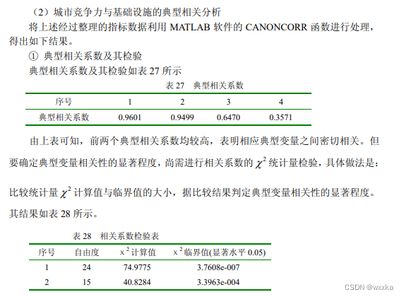
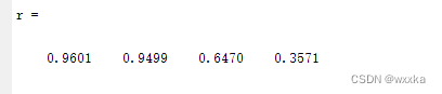
对于matlab中的典型相关分析函数canoncorr(x,y)
chi-squared statistic:卡方统计量
[A,B] = canoncorr(X,Y) computes the sample canonical coefficients for the n-by-d1 and n-by-d2 data matrices X and Y. X and Y must have the same number of observations (rows) but can have different numbers of variables (columns). A and B are d1-by-d and d2-by-d matrices, where d = min(rank(X),rank(Y)). The jth columns of A and B contain the canonical coefficients, i.e., the linear combination of variables making up the jth canonical variable for X and Y, respectively. Columns of A and B are scaled to make the covariance matrices of the canonical variables the identity matrix (see U and V below). If X or Y is less than full rank, canoncorr gives a warning and returns zeros in the rows of A or B corresponding to dependent columns of X or Y.
[A,B,r] = canoncorr(X,Y) also returns a 1-by-d vector containing the sample canonical correlations. The jth element of r is the correlation between the jth columns of U and V (see below).
[A,B,r,U,V] = canoncorr(X,Y) also returns the canonical variables, scores. U and V are n-by-d matrices computed as
U = (X-repmat(mean(X),N,1))*A
V = (Y-repmat(mean(Y),N,1))*B
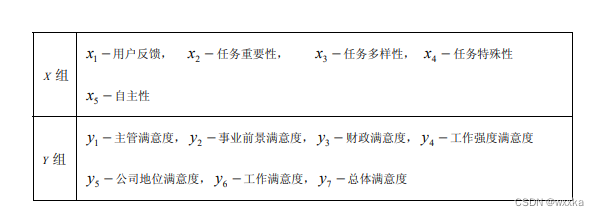
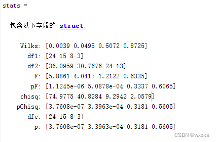
[A,B,r,U,V,stats] = canoncorr(X,Y) also returns a structure stats containing information relating to the sequence of d null hypotheses ![]() that the (k+1)st through dth correlations are all zero, for k = 0:(d-1). stats contains seven fields, each a 1-by-d vector with elements corresponding to the values of k, as described in the following table:
that the (k+1)st through dth correlations are all zero, for k = 0:(d-1). stats contains seven fields, each a 1-by-d vector with elements corresponding to the values of k, as described in the following table:
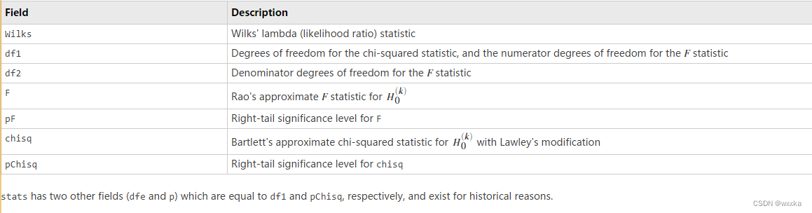
Wilks
Wilks' lambda (likelihood ratio) statistic
df1
Degrees of freedom for the chi-squared statistic, and the numerator degrees of freedom for the F statistic
df2
Denominator degrees of freedom for the F statistic
F
Rao's approximate F statistic for H(k)0
pF
Right-tail significance level for F
chisq
Bartlett's approximate chi-squared statistic for H(k)0 with Lawley's modification
pChisq
Right-tail significance level for chisq
stats has two other fields (dfe and p) which are equal to df1 and pChisq, respectively, and exist for historical reasons.
典型相关分析五部分:
1.指标相关性corrcoef
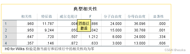
2.典型相关系数及检验
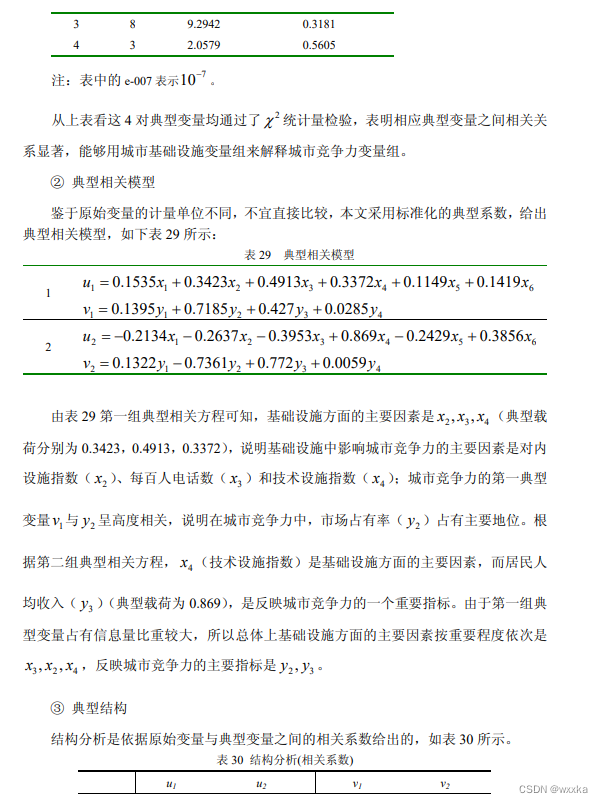
3.典型相关模型
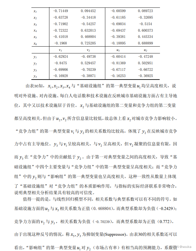
4.典型结构分析
5.典型冗余分析与解释能力


 1576
1576


 被折叠的 条评论
为什么被折叠?
被折叠的 条评论
为什么被折叠?
 到【灌水乐园】发言


