2.自用：重读大模型知识图谱融合《JointLK: Joint Reasoning with Language Models and Knowledge Graphsfor Commonsense》

之前就读过这篇文章，但文章对我来说犹如天书，经过几个月的学习（我很懒）重新看这篇文章，记录一下自己的学习过程，方便以后复盘。

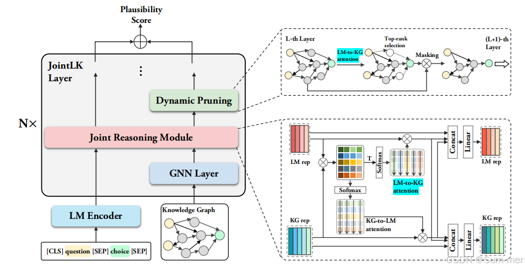
先看一张技术路线图，这个图已经把文章的框架讲的很清楚，有两大块：联合推理和动态修剪。

对于我而言问题在于：

如何读取知识图谱？

借助问题，我进行了以下学习：

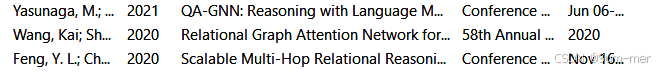
问题1：从图和文章可以知道GNN Layer主要作用就是作为一个KG的encoder，在文中3.3部分有具体介绍，bert获得实体表示，gnn更新节点表示，在附录a、b中有更详细的介绍。本文主要通过这三篇文章建立起方法：

通过笔记1，对Feng的文章进行理解，以下是对我来说帮助理解的要点：

一种简单的方法是直接利用知识图谱来建模这些关系路径，通过从知识图谱中提取关系路径并使用序列模型对其进行编码来模拟多跳关系	很难扩展，因为图中可能的路径数量（1）与节点数量呈多项式关系（2）与路径长度呈指数关系
图神经网络（GNNs）通过它们的信息传递公式具有更好的可扩展性，但通常缺乏透明度。变体（RGCNs和GCNs）	这些模型不能区分不同邻居或关系类型的重要性，因此无法为模型行为解释提供明确的关系路径。
本文：多跳图关系网络（MHGRN）	模型从GNNs那里继承了可扩展性，通过保持消息传递公式来实现这一点。同时，它还享受到了基于路径模型的解释性优势，方法是引入了结构化的关联注意力机制。

为了理解这篇文章，我觉得有必要去学习以下GNN，这里看的是b站上李沐老师讲的GNN文章。事与愿违，没有计算机背景的我根本听不懂，收获就是：原来图谱真的能输进去、原来真的可以做计算、而且还可以输出图。由于我不是计算机专业的，并且我的专业真不要求我搞懂，我决定放自己一马，不去深究了。

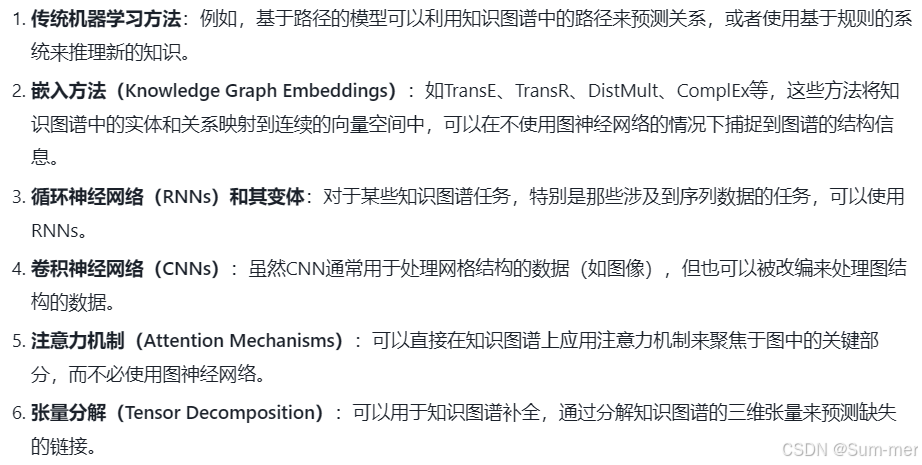
gnn属于图神经网络，可以有效学习知识图谱，但并不是只有图神经网络才能处理知识图谱：

回到原文提供的代码处，找到了该部分对应的代码：

class JOINTLK(nn.Module):
    def __init__(self, args, k, n_ntype, n_etype, sent_dim,
                 n_concept, concept_dim, concept_in_dim, n_attention_head,
                 fc_dim, n_fc_layer, p_emb, p_gnn, p_fc,
                 pretrained_concept_emb=None, freeze_ent_emb=True,
                 init_range=0.02):
        super().__init__()
        self.init_range = init_range

        self.concept_emb = CustomizedEmbedding(concept_num=n_concept, concept_out_dim=concept_dim,
                                               use_contextualized=False, concept_in_dim=concept_in_dim,
                                               pretrained_concept_emb=pretrained_concept_emb, freeze_ent_emb=freeze_ent_emb)
        self.svec2nvec = nn.Linear(sent_dim, concept_dim)

        self.concept_dim = concept_dim

        self.activation = GELU()

        self.gnn = QAGNN_Message_Passing(args, k=k, n_ntype=n_ntype, n_etype=n_etype,
                                        input_size=concept_dim, hidden_size=concept_dim, output_size=concept_dim, dropout=p_gnn)

        self.pooler = MultiheadAttPoolLayer(n_attention_head, sent_dim, concept_dim)

        self.fc = MLP(concept_dim + sent_dim + concept_dim, fc_dim, 1, n_fc_layer, p_fc, layer_norm=True)

        self.dropout_e = nn.Dropout(p_emb)
        self.dropout_fc = nn.Dropout(p_fc)

        if init_range > 0:
            self.apply(self._init_weights)

        self.mean_pooler = MeanPoolLayer()

    def _init_weights(self, module):
        if isinstance(module, (nn.Linear, nn.Embedding)):
            module.weight.data.normal_(mean=0.0, std=self.init_range)
            if hasattr(module, 'bias') and module.bias is not None:
                module.bias.data.zero_()
        elif isinstance(module, nn.LayerNorm):
            module.bias.data.zero_()
            module.weight.data.fill_(1.0)


    def forward(self, sent_vecs, concept_ids, node_type_ids, node_scores, adj_lengths, 
                adj, emb_data=None, cache_output=False, 
                batch=None, last_hidden_states=None, attention_mask=None):
        """
        sent_vecs: (batch_size, dim_sent)
        concept_ids: (batch_size, n_node)
        adj: edge_index, edge_type
        adj_lengths: (batch_size,)
        node_type_ids: (batch_size, n_node)
            0 == question entity; 1 == answer choice entity; 2 == other node; 3 == context node
        node_scores: (batch_size, n_node, 1)

        returns: (batch_size, 1)
        """
        gnn_input0 = self.activation(self.svec2nvec(sent_vecs)).unsqueeze(1) #(batch_size, 1, dim_node)
        gnn_input1 = self.concept_emb(concept_ids[:, 1:]-1, emb_data) #(batch_size, n_node-1, dim_node)
        gnn_input1 = gnn_input1.to(node_type_ids.device)
        gnn_input = self.dropout_e(torch.cat([gnn_input0, gnn_input1], dim=1)) #(batch_size, n_node, dim_node)


        #Normalize node sore (use norm from Z)
        _mask = (torch.arange(node_scores.size(1), device=node_scores.device) < adj_lengths.unsqueeze(1)).float() #0 means masked out #[batch_size, n_node]
        node_scores = -node_scores
        node_scores = node_scores - node_scores[:, 0:1, :] #[batch_size, n_node, 1]
        node_scores = node_scores.squeeze(2) #[batch_size, n_node]
        node_scores = node_scores * _mask
        mean_norm  = (torch.abs(node_scores)).sum(dim=1) / adj_lengths  #[batch_size, ]
        node_scores = node_scores / (mean_norm.unsqueeze(1) + 1e-05) #[batch_size, n_node]
        node_scores = node_scores.unsqueeze(2) #[batch_size, n_node, 1]


        mask = torch.arange(node_type_ids.size(1), device=node_type_ids.device) >= adj_lengths.unsqueeze(1) #1 means masked out

        mask = mask | (node_type_ids == 3) #pool over all KG nodes
        mask[mask.all(1), 0] = 0  # a temporary solution to avoid zero node [10, 200]
        # [[ True, False, False, False, False, False, False, False, False, False,
        # False, False, False, False, False,  True,  True,  True,... False是真节点

        gnn_mask = torch.arange(node_type_ids.size(1), device=node_type_ids.device) <= adj_lengths.unsqueeze(1) #1 means masked out
        # [10, 200]
        # [ True,  True,  True,  True,  True,  True,  True,  True,  True,  True,
        #  True,  True,  True,  True,  True True是真节点
        ### [5,150,200]hidden_transform-->svec2nvec
        last_hidden_states = self.activation(self.svec2nvec(last_hidden_states))

        gnn_output, new_mask, batch = self.gnn(gnn_input, adj, node_type_ids, node_scores, 
                                    batch=batch, gnn_mask=gnn_mask.to(node_type_ids.device),
                                    last_hidden_states=last_hidden_states, 
                                    lm_mask=attention_mask)
        # gnn_output:[10, 119, 200], new_mask:[10, 119], batch:[1190]
        # new_mask: tensor([[False, False, False, False, False, False, False, False, False, False,
        # False, False, False, False, False, False, False, False, False是假节点
        pool_mask=~new_mask
        # [10, 119]
        # [ True,  True,  True,  True,  True,  True,  True,  True, False,  True,
        #  True,  True,  True, False, False, False, False, 

        Z_vecs = gnn_output[:,0]   #(batch_size, dim_node)

        sent_vecs_for_pooler = sent_vecs

        pool_attn=None
        graph_vecs, pool_attn = self.pooler(sent_vecs_for_pooler, gnn_output, mask=pool_mask)

        if cache_output:
            self.concept_ids = concept_ids
            self.adj = adj
            self.pool_attn = pool_attn

        concat = self.dropout_fc(torch.cat((graph_vecs, sent_vecs, Z_vecs), 1))
        logits = self.fc(concat)

        return logits, pool_attn

我当然得借助人工智能理解一下了：

工作原理:

1. 概念嵌入: 将知识图谱中的概念编码成低维向量。
2. 文本编码: 将文本序列编码成低维向量，并将其转换成与概念嵌入维度相同的向量。
3. GNN 编码: 使用 GNN 网络对知识图谱进行编码，提取知识图谱中的结构信息。
4. 注意力池化: 使用注意力池化操作将文本和知识图谱信息进行融合，得到融合后的文本表示。
5. 全连接层: 使用全连接层对融合后的信息进行分类或回归预测。
6. 输出: 输出推理结果。

总结:

JOINTLK 模块是 JointLK 模型的主体部分，负责将文本和知识图谱信息进行融合并进行推理。它通过 GNN 网络和注意力池化操作有效地提取了文本和知识图谱中的信息，并结合全连接层进行分类或回归预测，从而实现了对常识推理任务的建模。

代码中的GNN层长这样：

self.gnn = QAGNN_Message_Passing(args, k=k, n_ntype=n_ntype, n_etype=n_etype,
                                        input_size=concept_dim, hidden_size=concept_dim, output_size=concept_dim, dropout=p_gnn)

回到之前定义的QAGNN_Message_Passing类中，我又借助人工智能理解了一下：

2. 编码器:

• emb_node_type: 节点类型嵌入层，将节点类型编码成低维向量。
• emb_score: 节点得分嵌入层，将节点得分编码成低维向量。
• edge_encoder: 边特征编码层，将边类型和节点类型编码成低维向量。

3. GNN 层:

• gnn_layers: GNN 层的列表，每个层都使用 GATConvE 算法进行消息传递。
• SAGPools: SAGPool 层的列表，用于对子图进行池化操作。

4. 注意力机制:

• SKatts: CQAttention 层，用于计算 LM 到 KG 的注意力权重。
• KSatts: CQAttention 层，用于计算 KG 到 LM 的注意力权重。

5. 其他参数:

• activation: 激活函数，使用 GELU。
• dropout: Dropout 层，用于防止过拟合。
• pooling_ratio: SAGPool 的池化比率。

6. 消息传递过程:

• mp_helper: 辅助函数，用于执行消息传递过程。
• forward: 前向传播函数，输入节点特征、边信息、节点类型和节点得分，输出更新后的节点特征和节点掩码。

7. 注意力机制和池化:

• 在每个 GNN 层中，模型使用 SKatts 和 KSatts 计算 LM 到 KG 和 KG 到 LM 的注意力权重，并将注意力信息融合到节点特征中。
• 在每个 GNN 层之后，模型使用 SAGPool 对子图进行池化操作，保留重要的节点，减少模型复杂度。

总结:

QAGNN_Message_Passing 模块是 JointLK 模型中用于进行图神经网络消息传递的核心模块。它通过 GATConvE 算法进行消息传递，并结合注意力机制和池化操作，有效地提取了子图中的知识信息，为后续的推理过程提供了支持。

我把关注放在了第三点，对应的代码是：

 self.gnn_layers = nn.ModuleList([GATConvE(args, hidden_size, n_ntype, n_etype, self.edge_encoder) for _ in range(k)])

gnn_layers: GNN 层的列表，每个层都使用 GATConvE 算法进行消息传递。

因此什么是GATConvE:   GATConvE是一种用于知识图谱嵌入（Knowledge Graph Embedding）的模型，它是基于图注意力网络（Graph Attention Networks, GAT）和卷积操作的结合。GATConvE模型主要用于处理知识图谱中的实体和关系，将其转化为低维空间中的向量表示，以便于进行各种下游任务，如链接预测、实体识别等。

在提供的代码最后也写了对其的定义：

class GATConvE(MessagePassing):
    """
    Args:
        emb_dim (int): dimensionality of GNN hidden states
        n_ntype (int): number of node types (e.g. 4)
        n_etype (int): number of edge relation types (e.g. 38)
    """
    def __init__(self, args, emb_dim, n_ntype, n_etype, edge_encoder, head_count=4, aggr="add"):
        super(GATConvE, self).__init__(aggr=aggr)
        self.args = args

        assert emb_dim % 2 == 0
        self.emb_dim = emb_dim

        self.n_ntype = n_ntype; self.n_etype = n_etype
        self.edge_encoder = edge_encoder

        #For attention
        self.head_count = head_count
        assert emb_dim % head_count == 0
        self.dim_per_head = emb_dim // head_count
        self.linear_key = nn.Linear(2*emb_dim, head_count * self.dim_per_head)
        self.linear_msg = nn.Linear(2*emb_dim, head_count * self.dim_per_head)
        self.linear_query = nn.Linear(1*emb_dim, head_count * self.dim_per_head)

        self._alpha = None

        #For final MLP
        self.mlp = torch.nn.Sequential(torch.nn.Linear(emb_dim, emb_dim), torch.nn.BatchNorm1d(emb_dim), torch.nn.ReLU(), torch.nn.Linear(emb_dim, emb_dim))


    def forward(self, x, edge_index, edge_type, node_type, node_feature_extra, return_attention_weights=False):
        # x: [N, emb_dim]
        # edge_index: [2, E]
        # edge_type [E,] -> edge_attr: [E, 39] / self_edge_attr: [N, 39]
        # node_type [N,] -> headtail_attr [E, 8(=4+4)] / self_headtail_attr: [N, 8]
        # node_feature_extra [N, dim]

        #Prepare edge feature
        edge_vec = make_one_hot(edge_type, self.n_etype +1) #[E, 39]
        self_edge_vec = torch.zeros(x.size(0), self.n_etype +1).to(edge_vec.device)
        self_edge_vec[:,self.n_etype] = 1

        head_type = node_type[edge_index[0]] #[E,] #head=src
        tail_type = node_type[edge_index[1]] #[E,] #tail=tgt
        head_vec = make_one_hot(head_type, self.n_ntype) #[E,4]
        tail_vec = make_one_hot(tail_type, self.n_ntype) #[E,4]
        headtail_vec = torch.cat([head_vec, tail_vec], dim=1) #[E,8]
        self_head_vec = make_one_hot(node_type, self.n_ntype) #[N,4]
        self_headtail_vec = torch.cat([self_head_vec, self_head_vec], dim=1) #[N,8]

        edge_vec = torch.cat([edge_vec, self_edge_vec], dim=0) #[E+N, ?]
        headtail_vec = torch.cat([headtail_vec, self_headtail_vec], dim=0) #[E+N, ?]
        edge_embeddings = self.edge_encoder(torch.cat([edge_vec, headtail_vec], dim=1)) #[E+N, emb_dim]

        # remove self loops
        edge_index, _ = remove_self_loops(edge_index)
        #Add self loops to edge_index
        loop_index = torch.arange(0, x.size(0), dtype=torch.long, device=edge_index.device)
        loop_index = loop_index.unsqueeze(0).repeat(2, 1)
        edge_index = torch.cat([edge_index, loop_index], dim=1)  #[2, E+N]

        # x = torch.cat([x, node_feature_extra], dim=1)
        x = (x, x)
        aggr_out = self.propagate(edge_index, x=x, edge_attr=edge_embeddings) #[N, emb_dim]
        out = self.mlp(aggr_out)

        alpha = self._alpha
        self._alpha = None

        if return_attention_weights:
            assert alpha is not None
            return out, (edge_index, alpha)
        else:
            return out


    def message(self, edge_index, x_i, x_j, edge_attr): #i: tgt, j:src

        assert len(edge_attr.size()) == 2
        assert edge_attr.size(1) == self.emb_dim
        assert x_i.size(1) == x_j.size(1) == 1*self.emb_dim
        assert x_i.size(0) == x_j.size(0) == edge_attr.size(0) == edge_index.size(1)

        key   = self.linear_key(torch.cat([x_i, edge_attr], dim=1)).view(-1, self.head_count, self.dim_per_head) #[E, heads, _dim]
        msg = self.linear_msg(torch.cat([x_j, edge_attr], dim=1)).view(-1, self.head_count, self.dim_per_head) #[E, heads, _dim]
        query = self.linear_query(x_j).view(-1, self.head_count, self.dim_per_head) #[E, heads, _dim]


        query = query / math.sqrt(self.dim_per_head)
        scores = (query * key).sum(dim=2) #[E, heads]
        src_node_index = edge_index[0] #[E,]
        alpha = softmax(scores, src_node_index) #[E, heads] #group by src side node
        self._alpha = alpha

        #adjust by outgoing degree of src
        E = edge_index.size(1)            #n_edges
        N = int(src_node_index.max()) + 1 #n_nodes
        ones = torch.full((E,), 1.0, dtype=torch.float).to(edge_index.device)
        src_node_edge_count = scatter(ones, src_node_index, dim=0, dim_size=N, reduce='sum')[src_node_index] #[E,]
        assert len(src_node_edge_count.size()) == 1 and len(src_node_edge_count) == E
        alpha = alpha * src_node_edge_count.unsqueeze(1) #[E, heads]
     
        out = msg * alpha.view(-1, self.head_count, 1) #[E, heads, _dim]
        return out.view(-1, self.head_count * self.dim_per_head)  #[E, emb_dim]

对于这段代码的解释：
代码主要步骤：

1. 准备边特征： 将边类型和节点类型编码成向量，并拼接在一起，作为边嵌入。
2. 处理自环： 移除自环，并添加自环的嵌入。
3. 节点更新：
   • 对节点表示和边嵌入进行线性变换，得到查询 (query)、键 (key) 和消息 (msg)。
   • 计算注意力分数，并进行 softmax 操作，得到注意力权重。
   • 根据注意力权重，对消息进行加权求和，得到更新后的节点表示。
4. MLP 层： 对更新后的节点表示进行多层感知器 (MLP) 操作，进一步融合节点特征。
5. 注意力权重： 可以选择返回注意力权重，用于可视化或分析。

代码中用到的 GNN 操作：

• 线性变换： 对节点表示和边嵌入进行线性变换，将它们映射到 GNN 隐藏状态空间。
• 注意力机制： 计算节点之间的注意力分数，并根据注意力分数对消息进行加权求和，实现节点表示的更新。
• 消息传递： 将更新后的节点表示传递给邻居节点，进行下一轮迭代。

 在解决问题的过程中，我意识到我对大模型微调知识理解浅薄，接下来将系统学习大模型微调知识；并且我还发现自己对文章代码中的各个文件的目的了解不清晰。